2 Why Classical Architecture Loops Strain
“Feedback is the control of a system by reinserting into the system the results of its performance. If these results are merely used as numerical data for the criticism of the system and its regulation, we have the simple feedback of the control engineers.”
— Norbert Wiener, Cybernetics (1948)
Author’s Note: Norbert Wiener, the founding father of cybernetics, established that true control requires feedback. In our context, this means that computer architecture is fundamentally a feedback loop, and our current crisis is simply that manual loops have become too slow to function effectively.
To understand how to design that loop, we must first make the pressure it faces explicit.
The crux
When architecture choices grow faster than trusted feedback, what must the loop record so AI helps rather than just adding more candidates?
Chapter 1 named Architecture 2.0 as a discipline for designing the design loop itself. It then made the claim concrete with a compact lighthouse prompt: design a low-power, RISC-V-based compute subsystem for real-time mobile XR under a 3 W, 3 nm-class mobile envelope, and return a design-space report with evidence and rejected alternatives. The prompt is intentionally small. The architecture state it implies is not.
This chapter explains why that state cannot be handled by merely asking a larger model to produce a larger answer. Computer architects already use models, simulators, benchmarks, profilers, spreadsheets, compilers, RTL flows, EDA tools, and expert reviews. The problem is not the absence of tools. The problem is that the design loop that coordinates those tools is under pressure. The space to search, the constraints to satisfy, and the evidence required to trust a result now grow faster than manual coordination, review, and verification capacity.
The claim is not that the old loop is obsolete. It is that the old loop must become a first-class object of design alongside the artifact it produces.
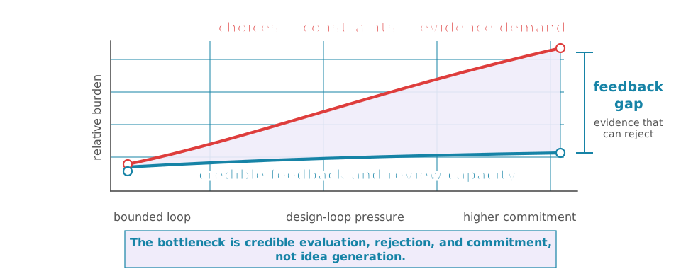
Scissors gap. The scissors gap is the widening gap between the rate at which design choices, constraints, and evidence demands expand and the rate at which a team can obtain trusted feedback, reject weak candidates, and commit responsibly.
The gap opens when the number of plausible actions, constraints, feedback sources, and evidence requirements grows faster than the loop’s ability to evaluate, reject, revise, and commit architecture candidates credibly. That is the visible failure mode. Trusted feedback cannot keep up with the choices and evidence demands the loop has created. For automation, the scissors gap sets the safe operating boundary. The loop can delegate only as much search, prediction, and synthesis as it can review and reject.
Architect’s checkpoint: The Delegation Gate
An automated method can only be delegated tasks where the loop has explicit, trusted rejection checks. If you cannot reject a bad candidate, you cannot safely delegate its generation.
The practical diagnostic is therefore not “where can we add a model?” It is “which part of the loop cannot keep up?” A loop may be representation-bound, action-bound, feedback-bound, rejection-bound, or commitment-bound. Each names a different part of the loop that saturates first, and each shows a different symptom, needs a different record to confirm, and calls for a different first fix (Table 2.1).
| Bound | Symptom | Lighthouse example | Record to inspect | First fix |
|---|---|---|---|---|
| Representation-bound | The loop cannot encode the state that decides the outcome, so it proposes candidates the environment later rejects. | It ranks XR compute organizations without representing memory-movement cost, so a later estimate overturns the proxy order. | The state schema: which fields the loop can read and write. | Add the missing fields (workload, interface, memory-traffic) to the representation. |
| Action-bound | The legal action set is too narrow, or too loose, to reach the candidate that would clear the gates. | The loop can retune parameters but cannot change the accelerator interface, so it never reaches the organization that would meet both the real-time deadline and the power envelope. | The action schema: which moves are legal, and recorded. | Widen or tighten the legal action set and record it in the loop contract. |
| Feedback-bound | Trusted feedback is too scarce or too expensive to keep up with the candidates generated. | Only a few simulation-stage estimates are affordable, so most candidates are dropped or committed unjudged. | The feedback budget and each check’s cost and fidelity. | Add cheaper proxies and a ladder of feedback fidelities so scarce feedback is spent where it changes a decision. |
| Rejection-bound | The loop generates faster than it can reject, so weak candidates survive to expensive stages. | Lacking a gate, an accelerator that leads a cheap proxy ranking is not rejected until an expensive check exposes its data-movement cost. | The rejection gates and the negative-trace log. | Add explicit gates and record every rejection with its reason. |
| Commitment-bound | The loop cannot say what evidence licenses which commitment, so it over- or under-commits. | A candidate clears both gates, but nothing states whether that authorizes more exploration or an implementation commitment. | The commitment boundary and the evidence level attached to it. | Set a commitment level the current evidence supports, and name what would raise it. |
Section 9.10 turns the rejection bound into a quantitative limit, but the pressure starts here. A loop that can generate faster than it can reject only widens the gap.
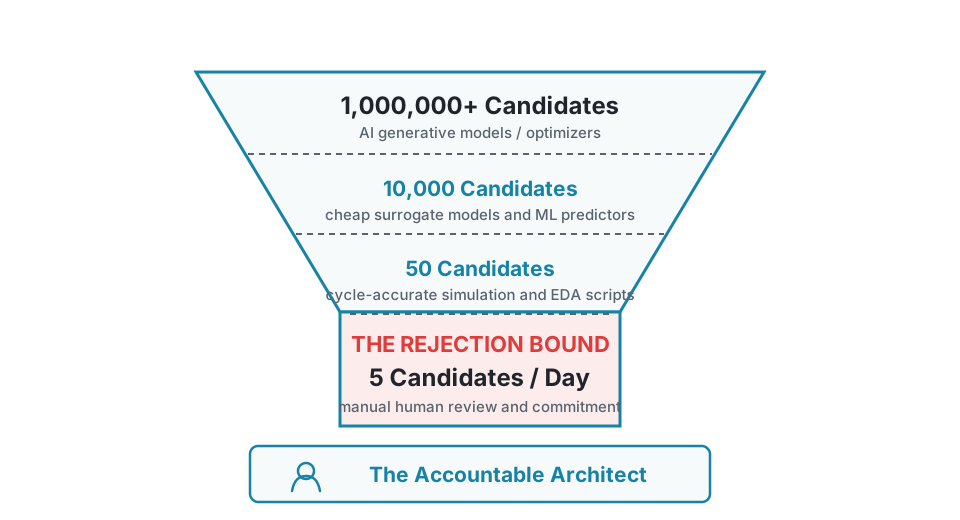
Because this failure mode is the central problem, the remainder of this chapter is not a general technology-trend survey. The pressures collapse into two fundamental limits: the Physical Wall (specialization, chiplets, memory movement, EDA) and the Verification Wall (software velocity, verification burden). They matter here specifically because they create that common failure mode. The fundamental economic logic of the loop is: generate cheap, reject expensive. The architecture team can imagine more candidates than it can evaluate, reject, and justify. Architecture 2.0 begins by making that failure mode explicit.
Read each section as a pressure test on one part of the loop. Cadence exposes gates and commitment policy. Architecture levers expand the state the loop must carry. Specialization and chiplets (multiple smaller dies integrated in one package) multiply actions. Software drift changes the workload contract. Physical constraints create early rejection conditions. Engineering cost makes feedback scarce. Generic AI assumptions fail because architecture work is not a cheap-label pipeline. Together, those pressures explain why the loop becomes a first-class architectural object alongside the artifact.
What this chapter gives you
After this chapter you can use the scissors gap to audit whether an AI-assisted architecture loop has enough trusted feedback to reject and commit responsibly. That means you can:
- recognize the scissors gap between choices and trusted feedback in a real architecture setting;
- explain why the bottleneck is trusted feedback, not idea generation;
- diagnose whether a loop is limited by representation, action validity, feedback, rejection, or commitment;
- point to the design and verification costs that make high-fidelity feedback scarce;
- connect each pressure source to loop state that can no longer remain implicit;
- identify where generic AI assumptions break at architecture boundaries;
- distinguish bounded AI roles from architect-owned commitment decisions.
2.1 Classical Loops Already Use Feedback
That first-class architectural object did not arrive out of nowhere; computer architecture has always been a loop. A typical loop begins with an intent: improve latency, reduce energy, raise throughput, support a workload, or fit a system into a power and cost envelope. The architect then chooses an abstraction, builds or selects a model, runs an analysis or simulation, studies the result, revises the design, and repeats. Eventually the work crosses into implementation, validation, verification, and signoff. That basic pattern is visible in textbook architecture practice and in industrial design loops (Hennessy and Patterson 2017).
Hennessy, John L., and David A. Patterson. 2017. Computer Architecture: A Quantitative Approach. 6th ed. Morgan Kaufmann.
A traditional SPEC CPU-style study makes the loop concrete. An architect might choose a subset of SPEC CPU workloads, propose a cache hierarchy or branch predictor change, run a simulator or performance model, inspect IPC, miss rates, branch-misprediction rates, area and power proxies, reject candidates that help one workload while hurting others, and repeat. Human judgment enters repeatedly: selecting workloads, deciding which proxy is credible, noticing unexpected behavior, choosing when a candidate is worth deeper analysis, and deciding which risk to accept. SPEC CPU 2017, for example, was designed as an industry-standardized suite for compute-intensive performance, stressing processor, memory subsystem, and compiler behavior (Standard Performance Evaluation Corporation 2017). The important point is not the specific suite version. It is the loop discipline: a bounded workload set, an explicit model, comparable metrics, rejection of weak candidates, and expert judgment about whether the evidence is strong enough.
Chapter 1 made the Architecture 1.0 to Architecture 2.0 loop shift visible in Figure 1.1. The point here is why that shift becomes necessary. Classical architecture loops already have intent, models, candidates, tool runs, and expert review. They strain when the state, action boundaries, evidence, rejection, and decision authority become too large to remain mostly implicit.
For the lighthouse prompt, the difference is not that Architecture 2.0 invents review discipline. The difference is what the loop must record before a result can be trusted. Table 2.2 summarizes that delta.
| Classical review might record | Architecture 2.0 additionally requires |
|---|---|
| Candidate design and measured result. | The represented task, workload slice, assumptions, and candidate provenance. |
| Tool output or benchmark score. | Tool version, heuristics, random seeds, feedback fidelity, uncertainty, cost, and what the feedback is allowed to reject. |
| Expert judgment about whether the result looks plausible. | Explicit rejection authority, failed or rejected candidates, and the commitment level the evidence supports. |
This loop is powerful because it does not require perfect automation. It combines formal models, approximations, domain knowledge, and review. It also rests on an unstated balance: the number of choices, the cost of evaluation, and the evidence needed to make progress must remain within the capacity of the team and tools. When that balance holds, the loop works. When it breaks, the team may still generate ideas, but it cannot evaluate and reject them fast enough to make credible progress. The loop contract of Chapter 1 is that balance written down and made visible.
2.2 Cadence and Gates Manage Risk
One way industrial practice has long held that contract together is by treating cadence itself as a loop policy. It limits which action class may change at a commitment boundary and defines the evidence needed to advance. Intel’s tick-tock model is the cleanest familiar example. A “tick” moved a known microarchitecture to a new process technology; a “tock” introduced a new microarchitecture on a more mature process. The point was not that product development was literally two steps. The point was risk isolation. Avoid changing every hard thing at once, preserve a cadence, and let evidence from one step inform the next. When node transitions lengthened, Intel described a move toward process-architecture-optimization, explicitly using longer-lived 14 nm and 10 nm process technologies while further optimizing products and processes to maintain product cadence (Intel Corporation 2016).
Intel Corporation. 2016. Intel Corporation 2015 Form 10-k. https://www.sec.gov/Archives/edgar/data/50863/000005086316000105/a10kdocument12262015q4.htm.
That history is useful for Architecture 2.0 because it shows that a design loop is not only a sequence of tools. It is also a policy for what is allowed to change, which evidence is strong enough to advance commitment, and how the organization reacts when feedback latency changes. Tick-tock separated process risk from microarchitecture risk. Process-architecture-optimization added an explicit optimization phase when process shrinks no longer arrived on the old schedule. Instead of every generation requiring both a new process step and a new architecture step, the loop could spend another cycle improving products, libraries, physical implementation, frequency, power, and yield on a known process. In other words, the cadence changed because the feedback and commitment costs of the physical process changed. Architecture 2.0 generalizes the same lesson. If AI methods increase the rate at which candidates are proposed, the loop must become stricter about change scope, evidence gates, rejection authority, and what kind of optimization is being performed.
Adjacent systems practices offer compatible lessons. EDA timing closure shows that a late tool can reject an early abstraction. The source-backed examples later in this chapter make the pattern concrete. Autotuning treats measurements as samples from a costly space, and benchmark governance depends on maintained rules and comparability contracts. A loop without observability, a decision policy, and escalation gates is not a credible loop. These analogies should not displace computer architecture. They help name the reusable loop properties architects already care about: cadence, state, feedback, gates, rejection, and commitment.
Autotuning: The process of automatically searching for optimal program or system parameters.
This is not the first time architecture has had to redesign its loop. Read the historical rows in Table 2.3 as examples of explicit action schemas, environment access, workload records, and rejection gates, not as a history survey. Each row names one kind of state, rule, or rejection path that would have to be exposed before an automated loop could help without weakening the evidence standard. The point is not nostalgia. The point is that many ideas that once looked unmanageable became tractable only after the field made some part of the loop explicit: the interface, the rules, the workload, the tool contract, the evidence gate, or the software path.
| Shift | What the loop made explicit | Architecture 2.0 lesson |
|---|---|---|
| System/360 compatibility | A stable ISA contract separated architecture from implementation across a product family (Amdahl et al. 1964). | Architecture is a durable interface and commitment policy, not only a circuit or microarchitecture. |
| Mead–Conway VLSI and MOSIS | Design rules, layout abstractions, and fabrication access turned custom-chip design into a shareable and reusable loop (Mead and Conway 1980; USC Information Sciences Institute 2025). | Representation and access to feedback can change who can participate in architecture work. |
| RISC | Workload, compiler, VLSI, and the quantitative Iron Law of Performance became the explicit architectural argument (Patterson and Ditzel 1980). | Evidence can reject attractive complexity when the full loop cost is visible. |
| SPEC-style benchmarking | Workload selection, run rules, reporting conventions, and comparability became community infrastructure (Standard Performance Evaluation Corporation 2017). | Benchmarks are loop governance, not just input programs. |
| Logic synthesis and timing closure | HDL, libraries, constraints, and timing reports gave downstream tools authority to reject upstream choices (De Micheli 1994). | Implementation feedback belongs in the architecture loop before commitment. |
| CUDA-style GPU programming | Kernels, thread hierarchies, memory spaces, libraries, and toolchains made specialized hardware programmable (Nickolls et al. 2008). | Specialized hardware succeeds only when the software loop is designed with it. |
Amdahl, Gene M., Gerrit A. Blaauw, and Frederick P. Brooks. 1964. “Architecture of the IBM System/360.” IBM Journal of Research and Development 8 (2): 87–101. https://doi.org/10.1147/rd.82.0087.
Mead, Carver, and Lynn Conway. 1980. Introduction to VLSI Systems. Addison-Wesley.
USC Information Sciences Institute. 2025. MOSIS 2.0’s First Year: Bridging Research and Production. https://www.isi.edu/news/972800/mosis-2-0s-first-year-bridging-research-and-production/.
Patterson, David A., and David R. Ditzel. 1980. “The Case for the Reduced Instruction Set Computer.” ACM SIGARCH Computer Architecture News 8 (6): 25–33. https://doi.org/10.1145/641914.641917.
Standard Performance Evaluation Corporation. 2017. SPEC CPU 2017 Benchmark. https://www.spec.org/cpu2017/.
De Micheli, Giovanni. 1994. Synthesis and Optimization of Digital Circuits. McGraw-Hill.
These examples should make the Architecture 2.0 claim less exotic. The field has repeatedly advanced by turning tacit craft into explicit loop structure. The new challenge is that AI methods can propose, search, summarize, and optimize at a scale that makes the loop state itself the bottleneck.
2.3 Architecture Levers Add State
That loop state did not appear all at once. It accumulated as architecture advanced by adding levers. For decades, technology scaling made the same basic design style better by providing smaller, faster, cheaper, and more energy-efficient transistors. Dennard scaling gave architects a favorable energy story as devices shrank (Dennard et al. 1974). As that story weakened, the field leaned harder on microarchitecture, instruction-level parallelism, caches, speculation, vector units, multicore, accelerators, specialization, and system-level optimization. The result is not a simple failure narrative. It is an accumulation of levers.
Dennard, Robert H., Fritz H. Gaensslen, Hwa-Nien Yu, V. Leo Rideout, Ernest Bassous, and Andre R. LeBlanc. 1974. “Design of Ion-Implanted MOSFET’s with Very Small Physical Dimensions.” IEEE Journal of Solid-State Circuits 9 (5): 256–68. https://doi.org/10.1109/JSSC.1974.1050511.
The accumulation matters because each lever creates both opportunity and obligation. Better microarchitecture adds policies and corner cases. Multicore adds coherence, synchronization, memory ordering, and workload partitioning. Specialization improves efficiency when the workload and software stack are understood, but it adds interfaces, data movement, programmability, and verification burden. Chiplets and heterogeneous integration promise modularity and scaling beyond a monolithic die, but they add partitioning, die-to-die interfaces, package-level constraints, test, yield, thermal coupling, and supply-chain questions.
Figure 2.1 summarizes the first part of the point. The field keeps adding levers because efficiency still matters. But the same moves that recover efficiency also increase the burden of representing the design state and producing trusted feedback.
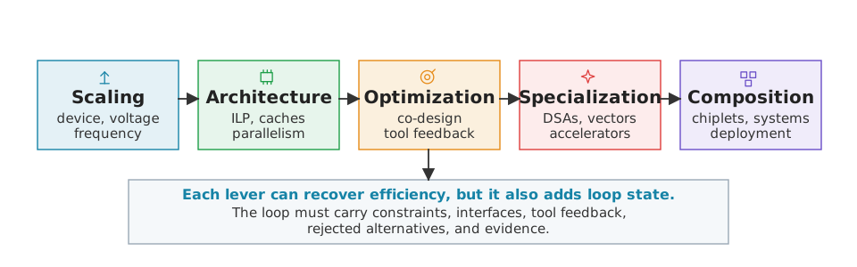
While Figure 2.1 illustrates a broad accumulation of design levers, the end of Dennard-style scaling and the limits of multicore scaling specifically explain why specialization became so central (Borkar and Chien 2011; Esmaeilzadeh et al. 2011). Hennessy and Patterson’s Turing Award lecture framed this moment as a new golden age for architecture, driven by domain-specific hardware/software co-design, open architectures, and agile hardware development (Hennessy and Patterson 2019). Architecture 2.0 should be read in that lineage, but with an explicit connection to the RISC revolution that preceded it. RISC was not just a simplified instruction set; it was the realization that making an architectural claim required a compiler, a benchmark, and a simulator. Architecture 1.0 gave us the tools to measure IPC and execution time, anchoring the field to the Iron Law of Performance (\(\text{Time} = \frac{\text{Instructions}}{\text{Program}} \times \frac{\text{Cycles}}{\text{Instruction}} \times \frac{\text{Time}}{\text{Cycle}}\)).
Borkar, Shekhar, and Andrew A. Chien. 2011. “The Future of Microprocessors.” Communications of the ACM 54 (5): 67–77. https://doi.org/10.1145/1941487.1941507.
Esmaeilzadeh, Hadi, Emily Blem, Renee St. Amant, Karthikeyan Sankaralingam, and Doug Burger. 2011. “Dark Silicon and the End of Multicore Scaling.” Proceedings of the 38th Annual International Symposium on Computer Architecture, ISCA ’11, 365–76. https://doi.org/10.1145/2000064.2000108.
Hennessy, John L., and David A. Patterson. 2019. “A New Golden Age for Computer Architecture.” Communications of the ACM 62 (2): 48–60. https://doi.org/10.1145/3282307.
Architecture 2.0 does not break the Iron Law; it uses the AI loop as an active co-designer to negotiate across the hardware-software boundary (compiler, ISA, microarchitecture), much like the early RISC teams did. The loop-level analogue is not the Iron Law but Amdahl’s. Chapter 9 shows that a design loop’s throughput is set by how cheaply it can reject, not by how many candidates it proposes, and derives that as a re-coordinatization of Amdahl’s law with trusted rejection as the serial fraction. Architecture 2.0 elevates the quantitative method from comparing candidate artifacts to designing the data, feedback, and evidence loops that make a larger, more coupled design space tractable. In that sense, the loop becomes a first-class architecture object: something to represent, instrument, test, reject, and improve.
That is the architectural consequence for Architecture 2.0. The new golden age gives the field more architectural levers; Architecture 2.0 asks how to govern the loop that uses them. Without that layer, AI assistance can only make the design space larger. With it, AI methods can be assigned bounded roles in search, evidence, rejection, and revision.
2.4 Specialization and Chiplets Expand Search
Of those bounded roles, search is the one most immediately stressed by the shift to Architecture 2.0, driven largely by the rise of specialization. Specialization is attractive because efficiency claims are multidimensional, the point Chapter 1 made explicit. The binding constraint differs across scales, from a battery- and thermally-limited mobile part to a warehouse-scale system bounded by power delivery and total cost of ownership (TCO) (Barroso et al. 2019). What this chapter adds is the consequence for the loop. Specialization does not just change which metric matters, it multiplies the decisions the loop must evaluate.
Barroso, Luiz André, Urs Hölzle, and Parthasarathy Ranganathan. 2019. The Datacenter as a Computer: Designing Warehouse-Scale Machines, Third Edition. Synthesis Lectures on Computer Architecture. Springer International Publishing. https://doi.org/10.1007/978-3-031-01761-2.
Specialization increases the number of architectural decisions because the architect must decide what to specialize, where to specialize it, and how it communicates with the rest of the system. A low-power XR subsystem is not just a choice between CPU and accelerator. It raises questions about vector length, memory hierarchy, local buffers, compression, dataflow, quantization, runtime scheduling, compiler support, sensor streams, display deadlines, thermal behavior, and fallback modes.
Chiplets compound the effect. They make it possible to compose systems from multiple dies and to mix process technologies, IP blocks, and memory technologies. But a chiplet system is not simply a bigger board-level system inside a package. The package changes latency, bandwidth, energy, thermal coupling, test, repair, physical constraints, and business boundaries. Open standards such as Universal Chiplet Interconnect Express (UCIe) aim to make die-to-die integration more composable by standardizing interface layers, protocols, software models, and compliance expectations (UCIe Consortium 2026). That standardization is valuable, but it also makes the architecture question more explicit: what should be partitioned, through which interface, under which evidence standard?
UCIe Consortium. 2026. UCIe Specifications. https://www.uciexpress.org/specifications.
The combinatorics are easy to understate. The following arithmetic is illustrative, not a measurement. Suppose a team is exploring only a narrow slice of the lighthouse prompt: an accelerator and memory subsystem for one workload family from XRBench (Kwon et al. 2023), a benchmark suite for extended reality systems. Even if it considers five compute organizations, four vector or accelerator interface choices, six memory hierarchy choices, four interconnect choices, three voltage/frequency policies, three compiler/runtime policies, and three verification or fidelity levels, the crude product is already:
\[ 5 \times 4 \times 6 \times 4 \times 3 \times 3 \times 3 \] That is 12,960 candidate loop states before workload versions, process corners, thermal constraints, reliability cases, and rejected configurations are counted. This number is intentionally conservative. More realistic architecture-adjacent loops quickly become much larger, or much slower, even before final silicon evidence is involved.
The product is also not just a counting problem. If each surviving state needs even a cheap analytical model, a simulator run, a synthesis check, or a human review, the loop is immediately limited by feedback cost and fidelity. Cheap models are essential, but they move the architecture problem rather than removing it. The loop must know when a proxy is good enough, when uncertainty is too wide, and when to escalate to stronger evidence. Chapter 4 turns that intuition into sample-cost and simulation-time representations, Chapter 5 separates feedback regimes by latency, fidelity, and rejection authority, and Chapter 6 returns to this same count in an evidence-gap plot that compares candidate scale with affordable high-fidelity samples.
In the Lighthouse slice, the same count is not search-space trivia. The CPU/accelerator/SoC choice also fixes interfaces, memory paths, compiler/runtime assumptions, physical constraints, and an evidence schedule: which states get cheap proxies, which get simulation, which escalate, and which rejected regions are preserved.
Engineer move: Triage a design-space slice before you simulate it
- Situation. A 12,960-state slice of the design space faces a fixed simulator-hour budget; not every state can be evaluated at full fidelity.
- Architecture decision. Which states get a cheap proxy, which get a cycle-level simulation, which escalate to stronger tools, and which regions to reject outright.
- Bound the loop. Fix the slice, the per-week simulator budget, and the metrics that decide the question (latency, energy, power).
- Method role. Use the AI system as a searcher and predictor. Rank states by a cheap proxy and propose the next most informative simulation. It proposes; it does not decide.
- Evidence path and escalation. Proxy-rank all states, simulate only the top candidates with logged provenance, and escalate to synthesis only after a candidate survives the cycle-level check.
- Negative trace. Record rejected regions with their reason (infeasible power, dominated latency) so the loop does not re-explore the same dead ends.
- Architect signs off. A human approves which surviving candidate has evidence strong enough for the next commitment, and owns the schedule risk if the proxy mis-ranked.
Beyond the lighthouse example, Table 2.4 grounds this combinatorial pressure in other concrete architecture settings. The examples are not meant to be a single measurement scale; they show that mapping, design-space exploration (DSE), physical design, and software tuning each impose a different kind of loop burden. Timeloop, an analytical framework for evaluating and mapping deep-neural-network (DNN) accelerators, makes the mapping case especially concrete. For a single convolutional-neural-network (CNN) layer with seven nested loop dimensions, mapped onto a four-level memory hierarchy, the number of legal mappings is astronomically large. Before hitting the raw math, consider what is being multiplied: for every level of the memory hierarchy, we must permute the order of the seven loop dimensions, and for every tensor, we must decide whether it bypasses each memory level. The exact expression matters less than its size. The unconstrained mapspace contains \((7!)^4 \times (2^4)^3\) arrangements before co-factor choices (such as tiling sizes) are even counted. The \((7!)^4\) factor counts loop-order permutations of the seven nested loop dimensions (e.g., batch, output channels, input channels, and spatial dimensions) at each of the four memory levels, and \((2^4)^3\) counts the level-bypass choices that decide which of the three tensors (inputs, weights, outputs) skip any of the four memory levels (Parashar et al. 2019).
Parashar, Angshuman, Priyanka Raina, Yakun Sophia Shao, et al. 2019. “Timeloop: A Systematic Approach to DNN Accelerator Evaluation.” 2019 IEEE International Symposium on Performance Analysis of Systems and Software, ISPASS, 304–15. https://doi.org/10.1109/ISPASS.2019.00042.
| Loop example | Scale anchor | Loop lesson |
|---|---|---|
| DNN accelerator mapping | Timeloop exposes loop permutations, factorization choices, and level-bypass alternatives. | Mapping is itself a combinatorial problem; architecture evaluation depends on the mapper and its constraints. |
| DNN accelerator DSE | MAESTRO, an analytical cost model for estimating DNN dataflow performance, reports 480M candidates, 2.5M valid designs, and 0.17M designs/s (Kwon et al. 2019). | Validity and pruning shape what evidence can be trusted. |
| TPU-block floorplanning | Learned floorplanning reported a months-to-hours loop compression; later work challenged baselines and reproducibility (Mirhoseini et al. 2021; Cheng et al. 2023). | High-fidelity tool feedback and rejection authority determine whether generation is credible. |
| Tensor-program tuning | AutoTVM, a machine learning-based tensor program optimizer, describes tensor-operator search spaces on the order of billions of possible implementations for a single GPU operator (Chen et al. 2018). | The software side of specialization also has a large hardware-dependent loop. |
Kwon, Hyoukjun, Prasanth Chatarasi, Michael Pellauer, Angshuman Parashar, Vivek Sarkar, and Tushar Krishna. 2019. “Understanding Reuse, Performance, and Hardware Cost of DNN Dataflows: A Data-Centric Approach.” Proceedings of the 52nd Annual IEEE/ACM International Symposium on Microarchitecture, MICRO ’52, 754–68. https://doi.org/10.1145/3352460.3358252.
Mirhoseini, Azalia, Anna Goldie, Mustafa Yazgan, et al. 2021. “A Graph Placement Methodology for Fast Chip Design.” Nature 594 (7862): 207–12. https://doi.org/10.1038/s41586-021-03544-w.
Cheng, Chung-Kuan, Andrew B. Kahng, et al. 2023. “Assessment of Reinforcement Learning for Macro Placement.” Proceedings of the 2023 International Symposium on Physical Design (ISPD). https://doi.org/10.1145/3569052.3578926.
Chen, Tianqi, Lianmin Zheng, Eddie Yan, et al. 2018. “Learning to Optimize Tensor Programs.” Advances in Neural Information Processing Systems 31.
The exact size of any one space is not the point. These examples differ in task, fidelity, and tool chain, but they share the same pressure pattern. Candidate count, validity, feedback cost, and evidence standards grow together. More candidates are useful only if the loop can evaluate, explain, and reject them (a dynamic we will formalize as the scissors gap in Figure 2.5).
2.5 Specialized Hardware Needs a Software Loop
The scissors gap is not solely a hardware problem. Specialization also exposes a software obligation. It is one thing to build an accelerator, vector unit, memory hierarchy, or chiplet partition that looks efficient in isolation. It is another thing to let programmers, compilers, runtimes, libraries, and deployment systems use it without destroying the efficiency claim through data movement, synchronization, code-generation overhead, or maintenance burden.
The historical examples in Table 2.3 show the same pattern. RISC depended on a compiler story. CUDA made GPU specialization useful by making the programming and toolchain loop explicit (Nickolls et al. 2008). The tensor-program row in Table 2.4 pushes the point further. Billion-scale operator search is already a software-side obligation of specialization. Systems such as Halide and MLIR, advanced compiler infrastructures used to define and schedule domain-specific operations, make scheduling, lowering, and intermediate representations central parts of the performance loop (Ragan-Kelley et al. 2017; Lattner et al. 2020).
Nickolls, John, Ian Buck, Michael Garland, and Kevin Skadron. 2008. “Scalable Parallel Programming with CUDA.” ACM Queue 6 (2): 40–53. https://doi.org/10.1145/1365490.1365500.
Ragan-Kelley, Jonathan, Andrew Adams, Dillon Sharlet, et al. 2017. “Halide: Decoupling Algorithms from Schedules for High-Performance Image Processing.” Communications of the ACM 61 (1): 106–15. https://doi.org/10.1145/3150211.
Lattner, Chris, Mehdi Amini, Uday Bondhugula, et al. 2020. “MLIR: A Compiler Infrastructure for the End of Moore’s Law.” arXiv Preprint arXiv:2002.11054, ahead of print. https://doi.org/10.48550/arXiv.2002.11054.
Field note: The architecture bet the compiler never paid: Itanium
Itanium’s EPIC architecture rested on one claim, that a compiler could statically expose enough instruction-level parallelism to feed a very wide machine (Schlansker and Rau 2000). Written as a design-loop card, that bet is a rejection gate waiting to fire.
- State seen: a wide static-issue target whose payoff needs sustained ILP close to the hardware’s issue width, running general-purpose code with unpredictable control flow and memory aliasing.
- Action allowed: widen the machine and delegate parallelism extraction to the compiler.
- Evidence required to commit: compiler-achieved ILP measured on representative branchy workloads, not the ILP the machine could retire in principle.
- Rejection rule: reject the wide-static bet if achieved ILP stays far below the issue width. The machine was built to issue on the order of six operations per cycle, against sustained integer ILP that real compilers struggled to push past one or two.
- Commitment owner: the architects who signed the tapeout.
The rejecting evidence was gatherable before commit by building the compiler, running real control flow, and measuring the ILP it actually extracts. Evaluated that way, the gate fires early and the bet is rejected in favor of a narrower or out-of-order organization. Instead the loop committed silicon on the assumed capability, and the part underdelivered against simpler rivals for a decade. Intel’s Larrabee made the same shape of bet a decade later, that software rasterization on many x86 cores would match fixed-function GPUs (Seiler et al. 2008), and Transmeta’s Crusoe bet that code-morphing software would let a simple core match x86 (Dehnert et al. 2003). Both rested on a software capability asserted rather than measured.
That is the whole difference. Architecture 1.0 can name this failure in hindsight.
Takeaway. Architecture 2.0 makes the compiler-ILP evidence a gate the bet must clear before commit, so an architecture can no longer be committed on a software capability that was asserted rather than measured.
Dehnert, James C., Brian K. Grant, John P. Banning, et al. 2003. “The Transmeta Code Morphing Software: Using Speculation, Recovery, and Adaptive Retranslation to Address Real-Life Challenges.” Proceedings of the International Symposium on Code Generation and Optimization (CGO), 15–24.
Seiler, Larry, Doug Carmean, Eric Sprangle, Tom Forsyth, et al. 2008. “Larrabee: A Many-Core X86 Architecture for Visual Computing.” ACM Transactions on Graphics 27 (3): 1–15. https://doi.org/10.1145/1360612.1360617.
Schlansker, Michael S., and B. Ramakrishna Rau. 2000. “EPIC: Explicitly Parallel Instruction Computing.” IEEE Computer 33 (2): 37–45.
For the lighthouse prompt, this means that a “64-bit RISC-V compute subsystem” cannot be judged by hardware structure alone. If the answer proposes a vector extension, custom accelerator, memory-local dataflow, or chiplet boundary, the loop must also represent how code reaches that mechanism, what compiler or runtime assumptions are required, which libraries or kernels use it, and which tests reject a design that is efficient only in a hand-written kernel. The software path is not downstream polish. It is part of the architectural claim. For an AI assistant, a hardware candidate is incomplete unless it also names the software contract and the tests that can reject unsupported semantics.
Lighthouse prompt: RISC-V is a software contract
Context. The ISA phrase fixes more than an instruction encoding. It names the boundary where AI-generated hardware choices become visible to compilers, runtimes, libraries, operating systems, and compatibility tests.
In the Lighthouse prompt. “64-bit RISC-V-based” and “vector-capable CPU, accelerator, or SoC block” make the software path part of the claim. An AI-assisted loop must explain how code reaches the mechanism, what ABI, memory-model, and toolchain assumptions it preserves, and what tests reject unsupported semantics.
Takeaway. The ISA is part of the evidence path for whether the AI-proposed subsystem can actually be used, not a label on the hardware box.
2.6 Software Changes Faster Than Silicon
Even when that software contract is perfectly specified, specialization still depends on stable enough targets. But modern software stacks move quickly. AI models change. Precision formats (e.g., FP8, INT4, block-scale formats1) and sparsity patterns (the structured or unstructured zeros in weights or activations that hardware can skip) mutate wildly, meaning the hardware must place bets on data types years in advance. Compiler passes change. Kernel libraries change. Runtimes, serving systems, quantization formats, batching strategies, fleet policies, and benchmark versions change. The hardware design cycle does not move at the same pace.
1 Block-scale formats share a single exponent across a block of low-precision mantissas to maintain dynamic range with minimal memory footprint.
Stack Overflow. 2024. 2024 Developer Survey. https://survey.stackoverflow.co/2024/.
Generative AI sharpens this mismatch rather than easing it. As models lower the marginal cost of producing code, the volume and churn of software rise rather than fall, a software-era instance of Jevons’ paradox. The shift is already visible in practice. By the mid-2020s, AI coding assistants had been adopted at scale. The 2024 Stack Overflow Developer Survey reported that a majority of professional developers were already using AI tools in their workflow (Stack Overflow 2024). The design target stops being a fixed workload an architect samples once and becomes the output of its own fast, semi-autonomous loop, retrained and regenerated faster than a hardware team can respond. A silicon program measured in years is then committed against a snapshot the software has already moved past. The architect cannot answer this by demanding faster silicon alone, because the fabrication cycle and physical closure set a floor on how short the hardware loop can be.
Jevons’ paradox: From nineteenth-century resource economics, the observation that making a resource cheaper to use can raise its total consumption instead of lowering it.
This forces a tradeoff the classical loop could often ignore. Peak efficiency comes from specialization, which is brittle when the workload drifts, while generality preserves agility at a cost in performance per watt. Under fast software churn, committing to a specialized design is a bet on workload stability, and that bet is increasingly made without evidence that the stability holds. The Architecture 2.0 response is not to abandon specialization but to make the bet explicit. Bound the workload the design serves, measure how fast it is drifting, and specialize only with evidence that the target will hold long enough to repay the silicon. That repayment includes the embodied carbon manufactured into the part up front, an irreversible commitment the holding workload must amortize, so a candidate that is low-energy in operation can still fail a carbon gate if the workload it bet on moves. The artifact remains the commitment target; the loop carries the evidence about whether the workload bet still holds.
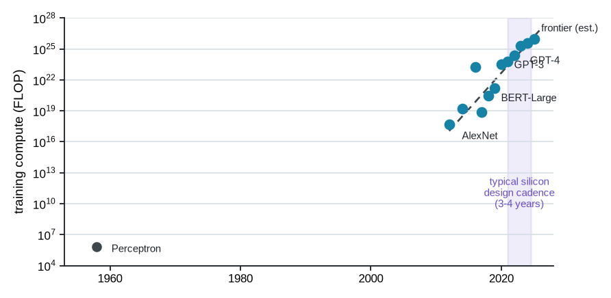
The scale of the target workload is not static either. For the loop, the important fact is not the compute-growth curve itself; it is that workload records expire. The compute behind notable AI systems has grown by roughly twenty orders of magnitude in nearly seven decades (Figure 2.2), so the workloads an architecture must serve can shift faster than a silicon program can absorb. A lighthouse loop should version model, compiler, runtime, benchmark, trace, and deployment snapshots, then trigger re-evaluation when drift crosses a commitment boundary.
Sevilla, Jaime, Lennart Heim, Anson Ho, Tamay Besiroglu, Marius Hobbhahn, and Pablo Villalobos. 2022. “Compute Trends Across Three Eras of Machine Learning.” arXiv Preprint arXiv:2202.05924. https://arxiv.org/abs/2202.05924.
This growing need to track moving workloads reflects a broader breakdown of abstractions, a shift that Compiler 2.0 offers as a useful adjacent warning. Amarasinghe’s framing is that compilers originally made hardware disappear for programmers, but multicore processors, vector instructions, accelerators, and heterogeneous systems have pushed more performance burden back onto programmers (Amarasinghe 2020, 2026). The same pattern appears at the architecture level. Abstractions still matter, but the design loop must now expose more of the workload, software, hardware, and physical state that earlier abstractions could hide.
Amarasinghe, Saman. 2020. “Compiler 2.0: Using Machine Learning to Modernize Compiler Technology.” Proceedings of the 21st ACM SIGPLAN/SIGBED Conference on Languages, Compilers, and Tools for Embedded Systems. https://doi.org/10.1145/3372799.3397167.
Amarasinghe, Saman. 2026. Compiler 2.0: Building the Next Generation Compilers with Machine Learning. https://www.csail.mit.edu/event/csail-forum-saman-amarasinghe-compiler-20-building-next-generation-compilers-machine-learning.
Mattson, Peter, Hanlin Tang, Gu-Yeon Wei, et al. 2020. “MLPerf: An Industry Standard Benchmark Suite for Machine Learning Performance.” IEEE Micro 40 (2): 8–16. https://doi.org/10.1109/MM.2020.2974843.
Reddi, Vijay Janapa, Christine Cheng, David Kanter, et al. 2020. “MLPerf Inference Benchmark.” 2020 ACM/IEEE 47th Annual International Symposium on Computer Architecture (ISCA), 446–59. https://doi.org/10.1109/ISCA45697.2020.00045.
Reddi, Vijay Janapa, Christine Cheng, David Kanter, Peter Mattson, Guenther Schmuelling, and Carole-Jean Wu. 2021. “The Vision Behind MLPerf: Understanding AI Inference Performance.” IEEE Micro 41 (3): 10–18. https://doi.org/10.1109/MM.2021.3066343.
To manage this rapidly changing software state, the community has had to formalize its workload agreements, making MLPerf a useful example. It was built to create common, reproducible machine-learning system benchmarks across a rapidly changing field (Mattson et al. 2020). MLPerf Inference sharpened the deployment-facing version of that problem. The paper reports more than 100 organizations building ML inference chips, systems spanning at least three orders of magnitude in power and five orders of magnitude in performance, and more than 600 reproducible measurements from 14 organizations in the first submission round (Reddi et al. 2020). The lesson is not only that benchmarks need rules. It is that a benchmark must encode scenarios, latency constraints, accuracy targets, software stacks, and comparability rules before performance numbers mean the same thing across systems (Reddi et al. 2021). That is also the challenge for architecture. A benchmark is not a fixed oracle. It is a maintained agreement about what evidence should count for a class of systems. The loop artifact is a versioned workload packet: traces, scenario constraints, acceptance tests, and expiration or review triggers.
For the lighthouse prompt, the workload is not merely “XR.” It is a moving bundle of sensing, perception, graphics, display, interaction, latency, quality-of-experience, and energy constraints. Even with XRBench (Kwon et al. 2023), a credible architecture loop must still decide which traces, model versions, deadlines, input distributions, and quality targets matter. If the software stack changes faster than the hardware loop can absorb, the design may optimize yesterday’s workload.
Kwon, Hyoukjun et al. 2023. “XRBench: An Extended Reality (XR) Machine Learning Benchmark Suite for the Metaverse.” Proceedings of Machine Learning and Systems.
2.7 Physical Constraints Move Into Architecture
Drifting workloads are only one source of pressure, pushing down from the software stack; physical limits push up on the loop from below just as hard. Architecture does not sit above physical reality. It is the layer where software intent, hardware mechanisms, and physical constraints become one design problem.
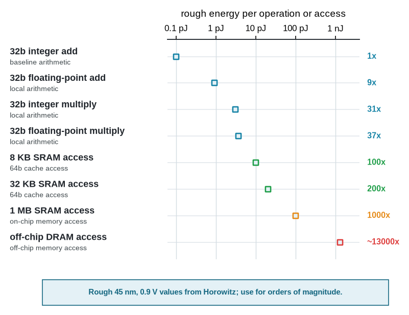
For example, data-movement estimates serve as early physical constraints, providing cheap rejection evidence rather than merely confirming that memory is expensive. Moving data through the memory hierarchy often costs far more energy than arithmetic, and Horowitz’s widely used energy estimates made this point concrete for a generation of architects (Horowitz 2014). That changes what architecture work means. A design loop cannot only ask which compute block is fastest. It must ask where the data lives, how often it moves, who schedules it, what locality exists, what precision is acceptable, and what the software stack can express.
Horowitz, Mark. 2014. “1.1 Computing’s Energy Problem (and What We Can Do about It).” 2014 IEEE International Solid-State Circuits Conference Digest of Technical Papers, 10–14. https://doi.org/10.1109/ISSCC.2014.6757323.
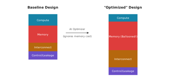
A useful architecture-level decomposition is \[ E_{\mathrm{system}} = E_{\mathrm{compute}} + E_{\mathrm{memory}} + E_{\mathrm{interconnect}} + E_{\mathrm{control}} + E_{\mathrm{leakage}} . \] This is not a circuit-level energy model. Use this decomposition as loop state. If any term is unrepresented, stale, or estimated outside its validity regime, the candidate should not cross the next commitment boundary. A candidate that reduces arithmetic but increases memory movement, interconnect traffic, control overhead, or leakage has not necessarily improved the system, a trade-off illustrated by Figure 2.3.
Interconnect costs have the same character as memory movement. On-chip networks, package links, memory interfaces, collectives, and host-device protocols define what a design can actually sustain. EDA and physical-design constraints also move upward. Timing, placement, routing, IR drop, thermal behavior, power delivery networks (PDN), leakage, signoff, and test are not late implementation details when they can overturn an architectural choice. Power and thermal density, for instance, can flag a dense accelerator mapping as risky early, and IR-drop and thermal signoff confirm or clear it later, once a placed netlist and current profile exist. Furthermore, because EDA tools rely on high-variance heuristics, a failed timing closure might just be a bad random seed, not a bad architecture. For a design loop, this means that a simulator score or model prediction is not enough. The loop needs a path from low-fidelity estimates to stronger evidence, and it needs rules for when physical constraints—or tool limitations—reject an otherwise promising candidate.
The Architecture 2.0 move is to make those physical assumptions inspectable before the loop delegates work. A generic generator can propose a faster block or a clever dataflow; an architecture loop must say which power model, memory traffic model, placement assumption, timing margin, and escalation rule make that proposal credible. Without that state, AI merely produces more candidates for a later physical-design step to reject. With that state, physical reality becomes an early design constraint, not a late surprise.
The important consequence is not that every early idea needs signoff-quality evidence. It is that the loop must know which physical assumptions are being made, what evidence would overturn them, and when to escalate from a proxy to stronger feedback. Otherwise the apparent speedup from AI-generated candidates is paid back later as discarded work.
The order-of-magnitude spread in Figure 2.4 is not something to memorize or treat as a current-node prediction. The architectural use is simpler. Local arithmetic and memory movement live on very different energy scales, so a loop that optimizes only arithmetic can improve the wrong thing. Advanced-node designs do not remove this lesson; if anything, the gap between local logic and moving data, driving wires, and feeding memory systems is one reason locality remains an architectural problem rather than a solved device-scaling detail. For the 3 nm-class lighthouse prompt, the loop would need a fresh power model before making a design decision.
The plot changes the section’s claim from “data movement is expensive” to “locality is an early rejection condition”. A loop that cannot represent memory movement cannot support a power or efficiency commitment.
2.8 Engineering Cost Creates the Scissors Gap
Each of these pressures, physical reality included, lands on the same fault line, a scissors gap. On one blade are design choices, workload variants, tool outputs, cross-layer assumptions, simulator hours, verification cases, EDA reports, physical constraints, and deployment signals. On the other blade are human attention, expert review time, tool budget, schedule, and verification capacity. The first blade rises quickly. The second does not.
Figure 2.5 makes the metaphor explicit. The upper blade is not only candidate count; it is the coupled burden of choices, constraints, evidence, software paths, and physical feasibility. The lower blade is not the ability to think; it is the slower-growing capacity to evaluate, review, reject, and commit with confidence.
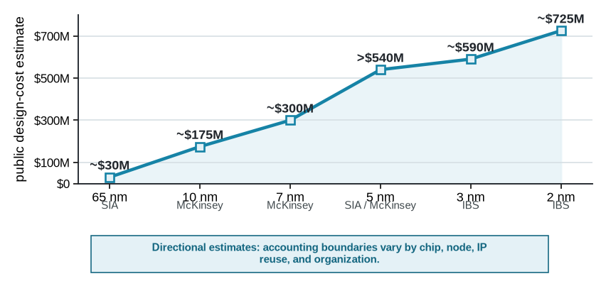
As a silicon-facing scale anchor, the gap is also an engineering-cost problem. Public estimates vary, and they should not be treated as universal accounting rules, but their scale is useful. The Semiconductor Industry Association reports that the cost of designing a latest-node chip rose from about $30M for a 65 nm chip in 2006 to more than $540M for a 5 nm chip in 2020, a greater than \(18\times\) increase (Semiconductor Industry Association 2026). A McKinsey analysis gives a similar order of magnitude, estimating roughly $175M for a 10 nm design, $300M for a 7 nm design, and $540M for a 5 nm design when validation, IP qualification, and related development costs are included (Bauer et al. 2020). These are not only mask or wafer costs. They are costs of architecture, design, validation, verification, IP, tools, and people.
Foster, Harry. 2022. Part 8: The 2022 Wilson Research Group Functional Verification Study. Verification Horizons, Siemens EDA. https://blogs.sw.siemens.com/verificationhorizons/2022/12/12/part-8-the-2022-wilson-research-group-functional-verification-study/.
Foster, Harry. 2025. IC/ASIC Functional Verification Trend Report - 2024. Verification Academy, Siemens EDA. https://verificationacademy.com/topics/planning-measurement-and-analysis/wrg-industry-data-and-trends/2024-siemens-eda-and-wilson-research-group-ic-asic-functional-verification-trend-report/.
Verification makes the people cost visible. In a summary of the 2022 Wilson Research Group functional-verification study, Foster reports that demand for IC/ASIC verification engineers grew faster than demand for design engineers from 2007 to 2022; the same summary reports that mean peak staffing is roughly one verification engineer per design engineer across most market segments, that processor projects can reach a 5-to-1 verification-to-design ratio, and that design engineers spent 49 percent of their time in verification in 2022 (Foster 2022). A later 2024 Wilson Research Group IC/ASIC report makes the commitment risk visible from another angle. It reports first-silicon success at 14 percent, the lowest level in two decades (Foster 2025). This is why feedback and rejection are central to Architecture 2.0. Each invalid candidate consumes scarce engineering capacity and commitment risk, not just compute cycles. This is the economic reason rejection, not generation, must pace automated search. Generated candidates are cheap only until they consume scarce verification, tool, and review capacity. ::: {.callout-field-note title=“The bug five entries wide: Pentium FDIV”} The 1994 Pentium FDIV bug cost Intel roughly $475M because five lookup-table entries were wrong, and no cheap check caught it before silicon.
Takeaway. The missing rejection, an automated gate that could have caught the error early, not the missing entries, set the price. ::: Figure 2.6 turns the public dollar estimates into a scale check. It should not be read as a universal cost curve. Different products, IP reuse strategies, node maturities, organizations, and accounting boundaries produce different numbers. The robust point is simpler. As the loop moves toward leading-edge implementation, feedback and commitment consume real engineering budgets, not only simulator cycles.
Semiconductor Industry Association. 2026. Chip Design and R&D. https://www.semiconductors.org/policies/chip-design/.
Bauer, Harald, Ondrej Burkacky, Peter Kenevan, Stephanie Lingemann, Klaus Pototzky, and Bill Wiseman. 2020. Semiconductor Design and Manufacturing: Achieving Leading-Edge Capabilities. McKinsey & Company report. https://www.mckinsey.com/industries/semiconductors/our-insights/semiconductor-design-and-manufacturing-achieving-leading-edge-capabilities.
International Business Strategies. 2024. Cost to Design an IC by Process Node. https://www.tomshardware.com/news/firm-estimates-a-2nm-chip-now-costs-dollar725-million-to-design.
The cost plot is not an indictment of architects. It says the unit of work has changed. The bottleneck is trusted feedback. That means preserving invalid candidates, proxy failures, assumptions, and the decision a human can responsibly commit to. Without that record, teams rerun old mistakes, rediscover invalid regions, and mistake more output for more architectural progress.
This bottleneck is not only a diagnosis. It has a bound. The diagnostic table earlier in this chapter asked which part of one loop saturates first; Chapter 9 makes the stronger, loop-wide claim precise. Whichever part saturates, end-to-end throughput is set by how cheaply the loop can reject, not by how much it can generate. Generating proposals faster than trusted feedback cannot keep up widens the scissors gap rather than closing it. Just as Amdahl’s Law dictates that sequential code bottlenecks multicore speedups, the Architecture 2.0 loop has its own Amdahl’s Law. No matter how fast the generative AI proposes candidates, the throughput of the design loop is bounded by the serial fraction of trusted, independent rejection capacity (see Figure 2.7). That capacity has two parts, and they age differently. How fast the loop can reject is a throughput limit, and cheap, independent, increasingly automated rejectors keep raising it. Who is accountable for the commitment if a claim is wrong is not a speed limit at all; it is a governance floor that stays human even as verification gets faster. Chapter 9 makes the throughput bound precise and shows how much of it an automated rejector can discharge before it reaches what only accountable judgment can clear.
2.9 Feedback and Verification Become the Bottleneck
That human review and rejection capacity is so strictly bounded because architecture feedback has uneven cost and uneven authority. A spreadsheet model is cheap but weak. A simulator may be more informative but slow or biased. A synthesis result exposes more implementation reality but depends on tool settings and constraints. Physical design and signoff are stronger still, but expensive and late. Silicon and deployment telemetry are authoritative in different ways, but they arrive after major commitments.
This feedback-regime structure makes naive autonomy dangerous. An optimizer that targets a cheap proxy may move quickly in the wrong direction. A search method that reports a Pareto frontier may hide invalid configurations, failed tool runs, or assumptions that would not survive signoff. A generated RTL fragment may look plausible but fail under verification or integration. Feedback becomes evidence only when its fidelity and provenance are clear, the discipline that Chapter 7 develops in full.
This is why Architecture 2.0 does not begin with autonomy. It begins with the loop. The loop must say what can be changed, what can be observed, what can reject a candidate, what evidence is strong enough for the next commitment, and what remains a human decision.
Architect’s checkpoint: The Automation Gate
When does an automated proxy ranking escalate to a human architectural decision? The loop must explicitly define which metrics, constraints, and failures require human signoff before the automated method can move a design to the next commitment level.
This discipline of designing the loop forces us to elevate feedback above generation, forming a core design principle for Architecture 2.0.
Design principle: Treat feedback as the bottleneck
More AI-generated candidates do not help a loop that cannot evaluate, reject, and justify them. Design for the rate of trusted feedback first, and add AI generation only as fast as human or automated rejection can keep up.
2.10 Architecture Violates Generic AI Assumptions
Designing a loop around the rate of trusted feedback is difficult exactly because architecture is not a standard machine-learning problem. Many successful AI systems are built in domains that generic machine-learning workflows take for granted, domains with abundant data, cheap feedback, stable labels, and clear losses. Those are exactly the conditions a design loop would want, and computer architecture violates them at almost every boundary. Data are often proprietary, incomplete, stale, or missing the rejected and failed candidates that explain why a design space has certain boundaries. Chapter 4 gives those records a sharper name and makes them part of loop state. Feedback ranges from a quick proxy to a simulation, synthesis run, physical-design report, expert review, emulation result, or silicon measurement, each with different latency, cost, fidelity, and authority. The action space is also unusual. Many generated configurations are not merely low quality; they are illegal, unsupported by tools, unverifiable, or incompatible with software and physical constraints.
The result is not a simple lack of data. It is a mismatch between generic AI assumptions and architecture-loop requirements. Architecture loops need representations that carry constraints, provenance, feedback cost, uncertainty, and rejection conditions. They also need methods that understand when a proxy result is only a proxy and when a decision is moving toward a higher commitment level.
A conventional machine-learning workflow is still useful as a foil. Students often learn a pipeline that runs from data collection to preprocessing, training, validation, deployment, and monitoring. Figure 2.8 keeps that familiar picture but shows why the architecture version cannot be a simple pipeline. Every step must carry validity constraints, tool costs, provenance, drift, rejected alternatives, and a commitment boundary.
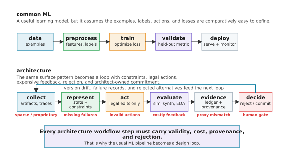
The mismatch has several concrete forms. Data are not just examples; they are design artifacts with permissions, tool versions, and missing failures. Feedback is not just a label; it spans regimes such as proxies, simulation, synthesis, physical design, expert review, emulation, and silicon. Actions are not just tokens; they are edits to configuration spaces, software interfaces, RTL, constraints, and deployment policies, many of which can be invalid. Losses are not just scalar rewards; they are multiobjective efficiency claims under performance, power, area, cost, reliability, sustainability, and verification burden. Table 2.5 gives the checklist version of that argument.
| Common AI assumption | Architecture violation | Loop implication |
|---|---|---|
| Abundant labeled data | Many labels are proprietary, expensive, stale, or not recorded. | The loop must build source records, provenance, and reusable failure records. |
| Cheap feedback | Simulation, synthesis, EDA, emulation, and review can be slow or scarce. | Methods must be sample-efficient and aware of feedback budgets. |
| Stable distribution | Workloads, software stacks, compilers, models, and deployment policies drift. | Benchmarks and representations must be versioned and revisited. |
| Valid actions are easy to define | Many generated configurations are invalid, unsafe, unverifiable, or unsupported by tools. | Environments need action schemas, constraint checks, and rejection authority. |
| Reward is clear | Efficiency mixes performance, energy, area, cost, reliability, sustainability, verification burden, and risk. | Objectives must be explicit, multiobjective, and tied to human decisions. |
| Proxy metrics are enough | Proxy wins can vanish at higher fidelity or under different workloads. | Evidence needs fidelity-regime checks and sensitivity checks. |
| Failures are just bad samples | Failed runs, rejected candidates, and invalid states describe the design space. | Failure records should be preserved as architecture data. |
This mismatch does not make AI irrelevant. It makes representation and loop design central. Architecture needs generation, prediction, optimization, critique, retrieval, and tool use. But those capabilities must operate inside an environment that knows what actions are legal, what feedback means, and who can say no.
2.11 AI Helps Only When the Loop Is Designed
If the environment can enforce those boundaries, AI becomes profoundly important because the classical loop is under pressure. It can help summarize tool outputs, propose candidates, search spaces, predict costs, construct tests, critique assumptions, retrieve prior designs, and coordinate subtasks. In domains with expensive feedback and large design spaces, even partial improvements in search, triage, and explanation can matter.
But AI is not sufficient because architecture is not only generation. The architectural problem is to produce a credible system artifact under constraints. That requires state, tools, evidence, rejection, and commitment. A model that proposes a design without exposing its assumptions has not solved the architecture problem. A loop that finds a better proxy score without recording rejected and failed candidates has not produced trusted evidence. A system that cannot say what rejects its own output cannot be given high-commitment authority.
The right conclusion is therefore narrower and stronger than generic AI optimism. We should not merely search larger design spaces. We should design loops that learn, record, reject, and justify architecture work.
2.12 Conclusion
This chapter asked what the loop must record, when architecture choices grow faster than trusted feedback, for AI to help rather than merely add candidates. The pressure is structural, not a matter of taste. Two walls converge on the classical loop. One is physical, built from specialization, heterogeneous integration, and data movement. The other is verification, built from software velocity and validation burden. Between them opens a scissors gap, in which generative methods raise the rate of plausible proposals far faster than any tool raises the rate of trusted rejection.
That reframes the problem. The scarce resource in modern architecture is not ideas but trusted feedback, the ability to evaluate, reject, revise, and commit at the fidelity a decision demands. An AI that widens the design space without widening rejection capacity makes the gap worse, not better. This is why feedback, not generation, sets the pace of progress, and why the chapter treats it as the bottleneck to design around.
AI assistance earns its place only inside a loop built to absorb it, one that records state, preserves failed and rejected candidates as evidence, names what can say no, and keeps a human accountable for each commitment. The goal is not a larger search space but a loop disciplined enough that more proposals become more progress instead of more noise.
2.13 Open Research Questions
The strain on classical design loops reveals that AI in architecture is not merely a generation problem, but a systems-design challenge. The following open questions highlight the research needed to make AI-assisted architecture reliable, verifiable, and capable of handling exploding design spaces.
For the strained-loop regime:
- The Minimum Inspectable Loop-State: How can we formally define the minimal state record—spanning task intent, action schemas, candidate provenance, and rejected alternatives—required to make an AI-generated architecture fully reviewable? As the scissors gap widens, this challenges the community to standardize the “black box” of AI generation so that human architects can securely audit and commit to designs even when high-fidelity samples are prohibitively scarce.
- Representing Failure and Uncertainty as Reusable Evidence: In the absence of abundant, open-source architectural data, how can a design loop safely internalize proprietary constraints, failed candidates, and tool-version drift? This requires pioneering new data representations that treat rejected designs and physical constraint violations (see the discussion on “Physical Constraints Move Into Architecture” in Section 2.7) not as wasted effort, but as mathematically rigorous negative evidence that prevents generative models from repeatedly exploring invalid regions.
- Provable Rejection Authority in the Scissors Gap: How can we construct a hierarchy of cheap, high-confidence rejection proxies that filter invalid AI-generated candidates before they consume validation cycles? Because feedback and validation are the ultimate limits on throughput (see the discussion on “Feedback and Verification Become the Bottleneck” in Section 2.9), discovering provably safe triage rules that minimize both false acceptances (which waste time) and false rejections (which discard optimal designs) is critical to scaling automated exploration.
- Versioning the Validity Horizon Against Software Drift: How must architectural claims be packaged to support reproducibility when software, models, and workloads mutate faster than the silicon design cycle (Section 2.6)? This invites the creation of dynamic, versioned workload snapshots and automated contracts between hardware commitments and software targets, so an AI-specialized architecture can trigger re-evaluation before a deployment bet becomes obsolete.
What to carry forward
- Reader test: When candidate scale and feedback cost grow together, can you say why trusted feedback, not idea generation, is the bottleneck, and what loop state the scissors gap demands?
- Up next: AI helps only when the loop records state, failures, evidence, rejection authority, and each commitment’s human owner; the discussion on “Architectural Claims and Design Loops” (Chapter 3) names the minimum loop state that makes that pressure inspectable.