9 Loop Patterns Across the Stack
“There is no single development, in either technology or management technique, which by itself promises even one order of magnitude improvement in productivity, in reliability, in simplicity.”
— Fred Brooks, No Silver Bullet (1986)
Author’s Note: Fred Brooks, Turing Award winner and author of The Mythical Man-Month, famously warned against hoping for a “silver bullet” in software engineering. For us, this is a reminder that there is no monolithic AI solution for the entire computing stack; instead, different layers—from compiler to RTL to SoC—require entirely different loop patterns.
The crux
The previous chapters built the components of an Architecture 2.0 loop, and Chapter 8 ran one bounded turn of it on the lighthouse prompt. We have seen one loop turn. Now we will map the five-part execution state onto three vastly different timescales: Software-defined (milliseconds), RTL/Simulation (hours), and Fleet (months). If the framework only describes one kind of design-space-exploration loop, it is too narrow. If it describes everything in the same way, it is too vague. The useful middle ground is a set of loop patterns.
Loop pattern. A loop pattern is a recurring shape of AI-assisted architecture work in which a generative method or automated optimizer acts on represented state under a characteristic feedback budget, evidence burden, rejection authority, and commitment level.
Workload characterization has one pattern. Fast compiler and runtime tuning has another. Accelerator, memory, interconnect, and chiplet exploration has another. Domain-specific architecture and code generation has another because local hardware efficiency only matters if the software path can reach it. Co-design across compute, memory, network, and power has another. Fleet and serving systems have another. RTL, physical design, and signoff have another. The ontology is the same, but the evidence burden changes.
This distinction protects the book from two mistakes. The first mistake is to pretend that every architecture task can be automated like a fast software loop. The second is to become so conservative that Architecture 2.0 is only a new name for old design review. The right question is more precise. Given this task, representation, environment, feedback budget, and commitment level, what method roles are useful, what evidence is credible, and what can reject the result?
What this chapter gives you
After this chapter you can choose the AI-assisted loop pattern before choosing the AI method. That means you can:
- classify an architecture task by its AI-assisted loop pattern and operating regime;
- compare cases with the same card fields instead of treating them as isolated anecdotes;
- name the cheap independent rejection authority and the human audit point for generative proposals;
- match the AI method posture and rejection authority to feedback cost and reversibility;
- state the unsupported claim boundary before the AI method overclaims.
9.1 A Template for Reading the Cases
The cases in this chapter are read through one card schema. The card asks for intent, task, design space, representation, environment, method role, feedback budget, evidence, negative traces, rejection authority, commitment boundary, and human decision. This keeps the chapter from becoming a list of examples. It also lets the reader compare loops that otherwise look unrelated. The lighthouse prompt remains the spine. When a separate benchmark, tool, or paper appears, it is used as a controlled slice of the prompt (workload coverage, code generation, architecture search, deployment feedback, or high-commitment physical evidence), not as a competing running example. The co-design pattern also carries the measured fleet-migration demonstration promised in Chapter 8.
Keep one rule in view as the cases become more technical. A loop does not scale because it can produce more candidates. It scales when the card can name a cheap, independent, trusted way to reject or clear a larger fraction of proposed commitments. The end of the chapter writes that rule as a bound, but the cases are the intuition for it.
To structure this intuition, Figure 9.1 maps out the chapter’s core spectrum, categorizing the loop patterns by their feedback latency and rollback cost. The boxes are not a maturity scale. Fast software loops are not better than high-commitment loops, and high-commitment loops are not more important than workload loops. They are different operating regimes for the same ontology.
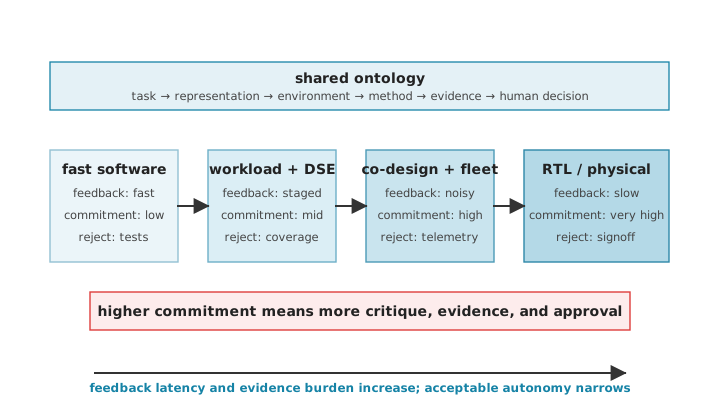
The figure should be read horizontally, not as a maturity ladder. A fast software loop may allow more automation because feedback is cheap and rollback is easy. A silicon-facing loop may use the same ontology but demands stronger evidence, independent rejection, and a tighter commitment boundary.
Table 9.1 provides the compact comparison across these regimes. The purpose is not to classify every paper perfectly. It is to force an Architecture 2.0 project to name its operating regime before choosing methods or making trust claims. Read the method column as an agency contract: what an assistant, optimizer, critic, or repair tool may do before independent evidence or a human owner can reject it.
| Loop pattern | Feedback and evidence | Useful method posture | Rejection and commitment |
|---|---|---|---|
| Workload and benchmark | Traces, benchmark versions, coverage, drift, and governance. | Generate, cluster, summarize, and test workload questions. | Reject through coverage gaps, leakage, or irrelevant metrics. |
| Fast software | Unit tests, compiler/runtime results, telemetry, and quick rollback. | Higher automation for bounded search, tuning, and repair. | Reject with tests, performance regressions, or deployment guards. |
| Architecture DSE and specialization | Simulators, proxies, surrogates, compiler/runtime paths, constraints, and Pareto evidence. | Generate candidates, predict, optimize, critique, and preserve negative traces. | Reject invalid actions, proxy mismatch, software incompatibility, or weak evidence. |
| Domain-specific architecture and code generation | Kernels, compiler IRs, libraries, runtimes, generated code, interface costs, and maintainability evidence. | Generate mappings, tune schedules, explain portability limits, and critique software-path gaps. | Reject local hardware wins that fail correctness, portability, interface cost, or deployment maintenance. |
| Co-design | Cross-layer models, workload traces, topology, memory, network, power, and thermal feedback. | Coordinate methods across layers and expose tradeoffs. | Reject single-layer wins that fail system objectives. |
| Systems and fleet | Deployment telemetry, canaries, drift, isolation, and operational constraints. | Adapt, monitor, critique, and revise policy under guardrails. | Reject with SLOs, safety policies, rollback, and human review. |
| RTL and physical | Formal checks, regressions, synthesis, timing, power, layout, signoff, and review. | Narrow search, organize evidence, critique, and repair bounded artifacts. | Reject with tool flows, signoff, and accountable architect-owned commitment. |
The cases that follow should be read through the same three questions. First, what are the physical constraints and rollback costs? A compiler flag, a runtime policy, an RTL edit, a chiplet boundary, and a fleet deployment do not carry the same blast radius (the scope of what a wrong change can damage). Second, what is the action-observation mapping? The loop should say what it can change and what tool, trace, log, or measurement it receives in return. Third, what are the rejection gates and human audit points? A case is not credible because it uses an advanced method. It is credible when the allowed actions, feedback source, evidence burden, and rejection authority match the commitment being made.
The rejection gate can also carry a blind spot that only scale reveals.
Field note: The cores that quietly did the math wrong
Takeaway. A rejection gate is only as good as the failure class it can see. At fleet scale the loop needs continuous, cross-checking rejection, because even the axiom every higher layer assumed, that the hardware computes correctly, is a claim that has to be verified.
For a new project, choose the loop pattern before choosing the method. Table 9.2 outlines the decision procedure for mapping a bottleneck to its corresponding loop pattern.
| If the bottleneck is… | Start with this loop pattern | First loop artifact or evidence ledger to build | Do not claim yet |
|---|---|---|---|
| Unknown workload coverage, stale benchmarks, or unclear scenario boundaries. | Workload and benchmark. | Versioned workload packet with coverage, gaps, and drift notes. | A general architecture win. |
| Fast code, compiler, runtime, or kernel feedback. | Fast software. | Testable code path with correctness, profiling, and rollback evidence. | Hardware/system superiority from a local speedup. |
| Many candidate architecture knobs under scarce simulation. | Architecture DSE and specialization. | Candidate records, action schema, proxy calibration, and rejected regions. | Implementation readiness. |
| Local hardware efficiency gated by software path, code generation, or interface cost. | Domain-specific architecture and code generation. | Executable software-path packet with kernels, IR/runtime path, interface-cost model, tests, and portability checks. | End-to-end architecture win. |
| Cross-layer tradeoffs across workload, compiler, memory, network, power, or deployment. | Co-design. | Interface map that names layer owners, changed assumptions, and rejection gates. | A single-layer optimum as a system result. |
| Live or deployment-like behavior, SLOs, canaries, or drift. | Systems and fleet. | Guarded telemetry packet with rollback and policy constraints. | Clean causal evidence without controls. |
| RTL, generators, physical design, signoff, or silicon-facing decisions. | RTL and physical. | Evidence ledger with tool-stage gates, waivers, and accountable review. | Autonomous commitment. |
9.2 AI-Assisted Loop Postures
Before traversing the stack layer by layer, it helps to classify AI-assisted architecture loops by structural shape. Despite operating on different parts of the stack, these loops share structural DNA, and they fall into three branches based on how the method interacts with the environment and the rejection authority: 1. The Surrogate Prediction Loop: The loop structure where the AI’s job is to replace a brutally slow Environment (like a 3-day EDA physical design run or full-system simulation) with a fast, differentiable proxy. The failure mode here is proxy mismatch, where the surrogate’s predictions diverge from the true physical constraints (such as predicting routing congestion, which is highly non-local and non-linear). 2. The Constrained Optimization Loop: The loop structure where the AI acts as the agent exploring a massively complex state space, heavily governed by a strict Rejection Authority. The environment itself is usually too complex to fully map, so the agent (often using Reinforcement Learning1) must discover paths that clear physics or timing gates. 3. The Generator-Critic Repair Loop: The loop structure where a weak generator (like an LLM2) proposes an artifact, fails a formal check, and uses the exact error trace as the next prompt. The rejection authority is absolute (e.g., a compiler or Verilator), and the loop iterates until the artifact parses or synthesizes correctly.
1 A machine learning method where an agent learns to make decisions by performing actions and receiving rewards or penalties.
2 Large Language Model, a neural network trained on vast amounts of text to understand and generate human-like language.
The chapter now walks the stack layer by layer. Each loop pattern below is an instance of one or more of these three branches, so when a new result appears, the useful question is not only which layer of the stack it touches but which branch of the loop taxonomy it is.
9.3 Workload Characterization and Benchmark Construction
Workload characterization is not a prelude to architecture work. It is architecture work. The workload defines what behavior matters, which metrics are meaningful, which software stack is assumed, and which design choices can be justified. Classic workload-characterization work made this concrete by measuring program behavior, comparing benchmark suites, and separating inherent workload properties from artifacts of a particular machine (Hoste and Eeckhout 2007). In Architecture 2.0, that lineage becomes loop state. Trace collection, benchmark construction, workload generation, clustering, summarization, coverage analysis, drift detection, and explicit questions about what the benchmark does not represent are all loop state.
The lighthouse prompt makes this concrete. “XRBench-class real-time mobile XR workload” is not a magic input string. XRBench gives the loop a benchmark anchor (Kwon et al. 2023), but the architecture question still depends on which XR workloads, models, devices, frame-rate targets, latency constraints, memory behaviors, and software paths are represented. A loop that optimizes one benchmark point may miss the distribution that a real mobile XR subsystem must serve. For an AI-assisted loop, the workload arrives as a packet, not a name. This packet includes scenario labels, device class, trace provenance, input distributions, excluded cases, coverage gaps, and rejection conditions.
MLPerf is the standing example; Chapter 2 treated it as maintained community infrastructure with versions, rules, and submission practices (Mattson et al. 2020). The point to carry into a loop pattern is not another benchmark history. The loop-pattern lesson is that a benchmark is a living agreement about what evidence should count. In the ML domain, workload drift is hyper-aggressive (e.g., shifting from dense Transformers to Mixture-of-Experts3 in months). A static benchmark quickly becomes a liability; an Architecture 2.0 loop must constantly ingest new computational graphs and trace data. A workload loop should therefore record benchmark version, workload source, coverage claims, known gaps, leakage risks, and the conditions under which a result should not generalize.
3 A neural network architecture where different parts of the model (experts) are activated conditionally based on the input, increasing capacity without a proportional increase in compute.
Table 9.3 makes this reframe explicit, contrasting traditional tasks with their Architecture 2.0 equivalents. The left column is still necessary: representative workloads, profiles, benchmark construction, and performance comparison remain central to architecture. The right columns state what changes when an automated optimizer is allowed to act inside the loop. The workload must become represented state, and the loop must know what evidence can reject a candidate that only wins a stale, narrow, or leaky workload slice.
| Architecture 1.0 meaning | Architecture 2.0 meaning | Loop state required | Failure if missing |
|---|---|---|---|
| Select representative workloads or benchmark suites. | Define the versioned workload distribution the loop is allowed to optimize over. | Scenario metadata, input distributions, versions, provenance, and inclusion/exclusion rationale. | The loop optimizes one stale or convenient slice and reports a false win. |
| Profile behavior: locality, branch behavior, memory traffic, bandwidth, latency, energy, and phase behavior. | Expose workload features that can drive prediction, search, critique, and active test selection. | Feature schema, measurement provenance, tool configuration, uncertainty, and known blind spots. | A predictor learns a proxy that does not survive another phase, input, or fidelity level. |
| Compare architectures under a fixed benchmark. | Maintain an evidence ledger across workload variants, candidate designs, and fidelity levels. | Candidate IDs, workload IDs, simulator/tool versions, feedback cost, accepted results, and rejected results. | Design-space results cannot be audited or reused by another loop. |
| Build or curate benchmarks for community comparison. | Define an environment contract: valid tasks, inputs, actions, metrics, leakage rules, and rejection checks. | Benchmark harness, validity checks, metric definitions, seeds, test splits, and update policy. | The loop overfits benchmark artifacts or takes actions outside the intended task. |
| Explain why a workload matters. | Make workload intent, deployment context, and drift explicit enough for a human to accept or reject decisions. | Use-case assumptions, deployment constraints, quality-of-service targets, telemetry hooks, and review notes. | The loop produces a plausible result for the wrong product or deployment regime. |
| Summarize results for a paper. | Preserve workload evidence as reusable architecture data. | Evidence ledger, negative traces, failed runs, rejected alternatives, and rationale for final claims. | The next loop repeats invalid experiments or loses why prior choices were rejected. |
The method roles in this loop are often not glamorous. A useful tool might cluster traces, generate candidate benchmark questions, identify missing coverage, compare workload versions, or critique whether a paper’s workload supports its claim. Those roles are valuable because they improve the question the architecture loop is answering.
Read as a loop card, the pattern is compact: the task is workload definition; the representation is versioned traces, metadata, and coverage notes; the environment is a benchmark harness with update rules; the method posture is clustering, summarization, generation of missing cases, and critique; the rejection authority is coverage, leakage, drift, or irrelevant metrics; the commitment boundary is whether a design claim may generalize beyond the measured slice.
9.4 Fast Software Loops
Moving from workload definition to code generation, fast software loops sit near the low-commitment end of the spectrum. Compiler flags, kernels, library implementations, runtime policies, configuration settings, and small code repairs can often be evaluated quickly and rolled back. Feedback may come from unit tests, microbenchmarks, integration tests, profilers, telemetry, or canary deployment.
Canary deployment: a controlled, partial rollout used to detect regressions before a system-wide release.
This is the regime where stronger automation is often plausible. Autotuning systems and learned tensor-program optimizers show how search spaces, cost models, measurements, and scheduling can be combined to improve software performance across targets (Chen et al. 2018; Zheng et al. 2020). An Architecture 2.0 loop can learn from that pattern without pretending that all hardware design is equally reversible.
Tensor-program optimizers: methods that automate the search for efficient execution schedules of tensor operations on target hardware.
Kernel-generation benchmarks make the same point in a current form. KernelBench evaluates whether models can produce GPU kernels that are both correct and faster than a baseline (Ouyang et al. 2025). This is a fast software loop because correctness tests, compilation, profiling, and microbenchmark feedback are close to the generated artifact. It also touches hardware/software co-design because performance depends on memory layout, parallelism, numerical precision, backend behavior, and target-specific hardware resources. Multi-platform kernel-generation work (often targeting intermediate frameworks like OpenAI’s Triton or CUDA) makes that bridge explicit by separating the core benchmark from target backends (Wen et al. 2025). For an automated optimizer, the benchmark object needs more than a prompt and a score: kernel IDs, input-shape distributions, correctness oracles, target metadata, compile/profile failure traces, and rejected variants.
Read as a loop card, the task is bounded code generation or tuning; the representation is source code, compiler IR, tests, target metadata, and profiling output; the environment is the compiler/runtime/profiler path; the method posture can be more automated because feedback is cheap; the rejection authority is correctness, compilation, portability, performance regression, and deployment maintainability; the commitment boundary arrives when a local kernel change becomes part of a larger software or hardware contract.
The reason autonomy can be higher here is not that the task is easy. It is that failures are often observable, bounded, and reversible. A generated kernel can be tested. A compiler flag can be reverted. A runtime policy can be canaried. A regression can be caught by a benchmark or deployment guard. Because rejection is close to the action, the loop can iterate quickly.
Failure mode: Fast feedback is not complete truth
9.5 Architecture Loops: Accelerators, Memory, and Chiplets
Moving beyond software, architecture design-space exploration represents the canonical middle case in terms of commitment and feedback cost. The loop may explore accelerator organization, vector width, cache hierarchy, local memory, interconnect, chiplet partitioning, and package assumptions. It may also choose how work is divided across CPUs, accelerators, and SoC blocks. Feedback is slower than software tests and less definitive than silicon. Actions can be invalid. Proxies can lie. The space is too large for exhaustive enumeration.
This is where the Architecture 2.0 framework feels most natural. The task is bounded but rich. The representation must expose architectural state. The environment must define legal actions and observations. Methods can generate candidates, predict behavior, optimize evaluations, critique assumptions, and preserve negative traces. ArchGym, an OpenAI Gym-based framework, is one example of making such loops more explicit for machine-learning-assisted architecture design (Krishnan et al. 2023); predictive design-space-exploration work shows that data-driven modeling has a longer architecture lineage (Ipek et al. 2006). Transferable frameworks such as Apollo go a step further, training a surrogate on an architecture dataset and carrying the same search across different design spaces (Yazdanbakhsh et al. 2021). That dataset has to be treated as a loop artifact, not a generic training set. Its design-space schema, sampled-region coverage, tool versions, invalid-action labels, rejected regions, and proxy-fidelity calibration determine what a generative method may infer from it.
Chiplets raise the stakes because they turn partitioning and interfaces into legal actions inside the loop. A UCIe-class interface should be represented as an environment contract that specifies what may be split across dies, what bandwidth/latency/power/thermal feedback tools return, which package and software assumptions are fixed, and which candidates must escalate or be rejected when interface evidence is missing (UCIe Consortium 2026).
Lighthouse prompt: The subsystem choice is an integration choice
In the Lighthouse prompt. “64-bit RISC-V-based compute subsystem” and “vector-capable CPU, accelerator, or SoC block” ask where the “XRBench-class real-time mobile XR workload” lives relative to the core, memory hierarchy, interconnect, compiler/runtime path, and product boundary. If the optimizer proposes a vector extension, it changes the CPU contract; if it proposes a tightly coupled accelerator, it changes the invocation, sharing, and memory-attachment contract.
Integration boundary. The method may still test a looser accelerator variant, but the loop environment must make the coupling assumption explicit so the optimizer cannot silently break integration contracts.
Architect’s checkpoint: The Cross-Layer Rejection Gate
Read as a loop card, the task is architecture search; the representation is candidate parameters, workload state, constraints, tool configurations, and prior rejected regions; the environment is a simulator, mapper, compiler path, or staged DSE harness; the method posture is generation, prediction, optimization, and critique; the rejection authority is invalid actions, simulator mismatch, power or software incompatibility, and weak Pareto evidence; the commitment boundary is escalation to stronger feedback.
9.6 Domain-Specific Architecture and Code Generation
When architecture search narrows to a specific problem, domain-specific architecture is often presented as an efficiency story. If the domain is narrower, the hardware can be more efficient. That statement is true but incomplete. A domain is not one knob. It can be a kernel family, a model family, a data type, a memory-access pattern, a programming model, a deployment regime, a latency envelope, a product vertical, or an ecosystem of libraries and tools. The golden-age argument for specialization (Hennessy and Patterson 2019) therefore creates a loop-design question. Which part of the domain is stable enough to specialize, and which part must remain programmable?
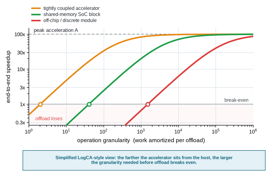
Use Amdahl here as a loop-contract check, not as an architecture refresher. The represented state is end-to-end workload fraction and offload granularity, the legal action is a specialization/interface choice, and the rejection rule is that a local speedup fails unless measured interface and software overheads still leave an end-to-end win. Every architect knows Amdahl’s law (Amdahl 1967), so restating it adds little. What follows is not a restatement but a relabeling of its variables. The version that matters here is the one that prices the interface. Hill and Marty re-derived the law for the multicore era to show how its lesson shifts when the substrate changes (Hill and Marty 2008), and LogCA, an analytical model for hardware accelerators, models the accelerator case directly. It makes offload latency, per-invocation overhead, and operation granularity first-class terms alongside the raw acceleration (Altaf and Wood 2017). The compact form used here keeps those costs visible: \[ S_{\mathrm{system}} \le \frac{1}{(1-f) + f/s + \epsilon_{\mathrm{interface}} + \epsilon_{\mathrm{software}}}. \] Here, \(f\) is the fraction of the end-to-end workload that the specialized mechanism can improve, \(s\) is its local speedup, and the \(\epsilon\) terms stand for the interface and software overheads that the LogCA-style model makes visible, expressed, like \(f\) and \(f/s\), as fractions of the baseline time so the terms share units. The reading is the one LogCA emphasizes. A design pays for specialization only when the accelerated work is large enough, and coarse enough per invocation, to amortize the cost of reaching the accelerator. A dramatic local speedup can still fail as an architecture result if the stable domain fraction is small, the interface is expensive, or the software path cannot keep up. This same form returns at the end of the chapter, lifted from one accelerator’s speedup to the throughput of the entire design loop (Section 9.10). For an AI-assisted loop, this equation is a rejection contract. A proposed specialization is not credible unless the method also carries interface, software-path, and end-to-end evidence.
To formalize this interface tax, Figure 9.2 uses a simplified LogCA-style calculation (Altaf and Wood 2017). End-to-end speedup is not a property of the accelerator alone. It rises with the work amortized per offload, and only after that granularity clears a break-even point set by offload latency and overhead. A tightly coupled unit breaks even at small granularity; an off-chip module may need thousands of operations per call before offload is worth doing at all.
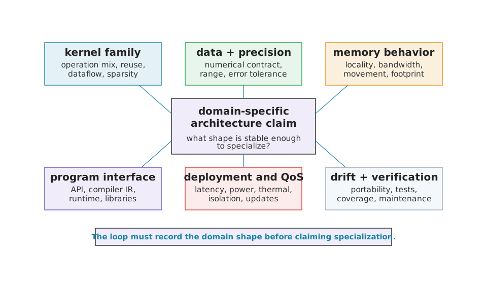
Consequently, Figure 9.3 breaks down the multidimensional nature of domain specificity. It should be read as a rigorous checklist rather than a simple taxonomy. Before a loop proposes a domain-specific block, it should say what shape of domain it is using and what that choice implies for representation, action space, evidence, and maintenance. A benchmark name is not enough. Two workloads in the same named domain may have different memory behavior, precision contracts, software interfaces, or deployment drift. The kernel family, precision contract, data-movement pattern, software interface, drift risk, and test coverage determine which optimizer actions are legal and which claims a loop must reject.
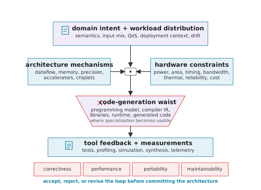
If the domain shape determines what to build, the software path is the loop’s narrow waist. Halide-style algorithm/schedule separation, AutoTVM/Ansor-style measured schedules, and MLIR-style multi-level compiler representations matter here because they turn software reachability into represented state, legal mapping actions, compiler feedback, and rejection evidence for specialized hardware claims (Ragan-Kelley et al. 2017; Chen et al. 2018; Zheng et al. 2020; Lattner et al. 2020).
To link these constraints, Figure 9.4 visualizes this software path, showing why code generation is the narrow waist of specialization. Above the waist are domain intent and workload distributions. Below the waist are hardware mechanisms, tool feedback, profiling, simulation, and deployment evidence. The waist itself contains the programming model, compiler IR, libraries, runtimes, and generated code that let the workload reach the machine.
Generative methods may help at this waist, but only inside a represented loop. Kernel-generation benchmarks are encouraging precisely because they keep correctness tests, compilation, profiling, and target-specific behavior close to the generated artifact (Ouyang et al. 2025; Wen et al. 2025). For architecture, the same discipline must extend beyond one kernel. The loop needs workload semantics, data layout, scheduling constraints, backend capabilities, correctness tests, portability limits, and rejection authority. The architectural question is not only whether a specialized block is efficient. It is whether the hardware/software interface can keep that efficiency usable as workloads, models, compilers, and products change.
Read as a loop card, the task is not “generate code” in isolation. It is to keep a domain-specific hardware claim executable. The representation includes domain shape, kernel family, compiler IR, runtime interface, data layout, and maintenance evidence. The feedback budget is split. Kernel and schedule feedback is cheap and reversible, so a method may tune aggressively at that level, while the hardware-interface commitment it implies is expensive and hard to undo, so the loop must hold that layer behind independent evidence. The rejection authority is correctness, portability, interface cost, workload drift, and end-to-end system measurement. The commitment boundary is the point where a cheap kernel-level win gets read as a hardware-interface decision, which only end-to-end measurement and a human owner may cross.
Architect’s checkpoint: The Hardware-Interface Commitment Gate
Failing to secure this commitment boundary often leads to a classic architectural trap, where localized optimizations fail to deliver expected end-to-end performance.
Failure mode: The accelerator that won in isolation
9.6.1 Progressive Lowering as the Architecture Loop
Treating the compiler merely as a “rejection gate”—a static wall the hardware bounces against—is an Architecture 1.0 mindset. In an Architecture 2.0 loop, the compiler is not a wall; it is the co-design engine. If the AI loop is exploring a reconfigurable spatial array or a custom vector accelerator, the instruction set is not static. The AI must synthesize the hardware and the compiler pass to target it simultaneously. The software contract isn’t a fixed boundary; it is a co-optimized variable.
This process is Progressive Lowering. When the AI agent decides to add a custom compute unit, it does not just output Verilog. It outputs Intermediate Representation (IR) dialects. It generates the new software dialect, the lowering rules to map high-level math into it, and the hardware dialect (using frameworks like CIRCT—Circuit IR Compilers and Tools—or MLIR) that implements it in silicon. The rejection authority is no longer just a simulator failing dynamically; it is the MLIR verifier proving statically that the lowering from software IR to hardware IR is semantically invalid (see Listing 9.1).
// Architecture 2.0 AI Loop Output: Co-generated HW and SW
// The agent writes the MLIR dialect and the lowering strategy simultaneously.

// 1. The AI defines the hardware intent using CIRCT (Hardware IR)
hw.module @CustomXR_SystolicArray(in %clk: i1, in %act: tensor<16x16xf16>, out %res: tensor<16x16xf16>) {
  // Agent-generated spatial architecture constraints
  %area_est = hw.predict_area(...)
  // Loop rejects if %area_est > mobile_XR_budget
  // Note: Area is heavily approximated here; true IR drop or routing congestion requires physical synthesis.
}

// 2. The AI simultaneously generates the compiler scheduling policy
// using MLIR Transform Dialect to map the XR workload to the new hardware
transform.sequence failures(propagate) {
^bb1(%arg1: !pdl.operation):
  // Agent discovers tiling to 16x16 is optimal for the power envelope
  %0, %loops:2 = transform.structured.tile %arg1 [16, 16]

  // Agent generates the mapping rule to the custom hardware it just designed
  transform.structured.map_to_custom_hw %0 { target = @CustomXR_SystolicArray }
}
9.7 Co-Design Loops: Compute, Memory, Network, and Power
While domain-specific loops focus on vertical execution, co-design loops test the oldest claim in this book. Architecture is not only a layer below software but the place where software behavior, hardware mechanisms, physical constraints, and system objectives meet. A single-layer optimization can therefore be locally correct and globally wrong.
Consider a dataflow choice that reduces compute cycles but increases memory traffic, a topology change that improves one collective while worsening another, a cache change that improves average performance but increases tail latency, or a rack-level policy that saves power while violating service quality. The loop must represent more than one layer because the objective lives across layers.
Energy and warehouse-scale coupling matter here because they give the loop cheap rejectors for cross-layer claims. Data movement, memory locality, network contention, power and thermal headroom, and deployment policy can all invalidate a local compute win before expensive implementation evidence is gathered (Horowitz 2014; Barroso et al. 2019).
An Architecture 2.0 co-design loop therefore needs richer representations, such as workload phase behavior, data movement, memory locality, network behavior, power and thermal constraints, compiler/runtime choices, and deployment policy. The useful method roles are coordination and critique as much as search. The loop should ask which layer changed, which objective improved, which objective worsened, and which evidence would reject a single-layer win. In an AI-assisted co-design loop, coordination means naming which layer the automated optimizer may touch, which layer supplies independent feedback, and which owner accepts the cross-layer tradeoff.
Architect’s checkpoint: The Cross-Layer Ownership Gate
Warehouse-scale computing itself, read as a loop card, is a cross-layer co-design pattern. The task is useful work per constrained resource; the representation is workload, software, hardware, network, power, cooling, and operations state; the environment combines models, traces, deployment measurements, and operational rules; and the rejection authority is a system objective that a local win violates.
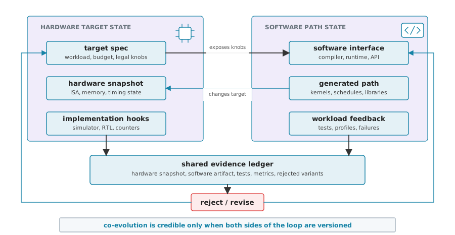
Many Architecture 2.0 loops are even less static than this summary suggests. In early accelerator, compiler, runtime, or system-interface work, the hardware target and the software path may both be changing. The loop is then not merely searching a fixed space; it is managing hardware/software co-evolution. A new instruction, tensor unit, scratchpad policy, data layout, or runtime interface changes what software can express, while compiler, kernel, and workload feedback changes which hardware feature is worth keeping. The evidence ledger has to record that co-evolution by tracking what hardware state existed when the software was generated, which examples or optimization rules were available, which correctness checks and performance measurements returned, and which hardware or software assumption was revised after rejection.
The durable lesson is not that code generation solves architecture. It is that software feedback can become part of architecture evidence when the loop keeps the hardware target, code path, tests, performance counters, rejected variants, and decision owner tied together. Without that record, a strong generated kernel or library path may only prove that one software artifact matched one hardware snapshot.
To manage this co-evolution, Figure 9.5 illustrates the rigorous loop discipline required to keep evidence aligned. Because the hardware side and software side may both change, so the evidence ledger must record the versions, measurements, failures, and rejected variants that connect them. Otherwise, the loop cannot say whether the architecture improved or only whether one generated path happened to work.
Google’s warehouse-scale migration from x86 to Arm is a deployed instance of this discipline (Christopher et al. 2025). It is not a hardware co-design loop. The target ISA is fixed, and the loop repairs software to meet it. But moving a production fleet of core services onto a new instruction set is a fleet-scale software-repair loop in which tens of thousands of applications must follow, and it is the book’s one measured exemplar; no measured cross-layer hardware co-design loop is offered. The reported effort analyzed more than 38,000 migration commits and wrapped part of the software change in an AI-assisted build-and-test repair loop, accepting a candidate fix only when the build and the test suite pass, and letting a fleet monitor automatically evict jobs that crash-loop or run slow on the new target. Authority sits with the instruments, not the generator. Build, test, sanitizers that expose memory-model differences between the two ISAs, and the production monitor that rejects regressions and preserves the evicted cases as negative traces for offline debugging. The repair tool resolves only a minority of failures on its own, roughly a third of broken tests without tuning, and the hardest changes stay with the application owners who know the code. The model behind the loop will age; the structure, a represented migration loop with instrument-held rejection authority and human-owned exceptions, is the part worth keeping.
When read through the same card, the migration case is not primarily an Arm story; it is a loop-contract story. Table 9.4 summarizes the reusable fields that structure this contract.
| Card field | Migration reading |
|---|---|
| Task | Move production services across an ISA boundary while preserving build, test, and rollout behavior. |
| Representation | Migration commits, build targets, tests, sanitizer findings, service ownership, and evicted production cases. |
| Environment | Build-and-test repair loop plus production monitoring on the new target. |
| Method role | Propose bounded software repairs and route failures toward owners. |
| Cheap independent rejector | Build failures, test failures, sanitizer failures, crash loops, slow jobs, and monitor-triggered evictions. |
| Commitment boundary | Automated repair can clear only the failures its instruments settle; application owners keep the exceptions. |
The most instructive result is what the evidence overturned. Going in, the team and the application owners expected the work to be dominated by low-level architectural differences like floating-point drift, concurrency, and platform-specific intrinsics. The recorded evidence showed otherwise. Most of the effort was tests that encoded x86-specific assumptions, build and release systems, and configuration rollout. Unaided architectural intuition mispredicted where the work actually was. That is the case for a represented, evidence-bearing loop in a single sentence. The loop found the work the experts did not expect.
Lighthouse prompt: Migration evidence shows what ISA claims owe
In the Lighthouse prompt. If the model chooses a “64-bit RISC-V-based” path for the “compute subsystem”, it means the AI-assisted loop owes evidence for generated code, ABI and memory-model assumptions, compiler/runtime behavior, library support, tests, and deployment rollout, not just an instruction encoding.
Boundary. The migration case is not the same target, but it reveals the kind of software-contract evidence a RISC-V subsystem claim would eventually need. Build, test, sanitizers, production monitors, and application owners become rejection authorities for the AI’s ISA choice.
Takeaway. ISA decisions proposed by an automated optimizer are credible only when the loop can show what software actually survives the contract and what remains a human-owned exception.
9.8 Deployment-Facing Architecture Loops: Runtime, Serving, and Datacenter Policy
Moving from design and migration to active operation, deployment-facing architecture loops evaluate architecture choices in deployed or deployment-like contexts. They include scheduling, serving, admission control, memory allocation, power management, placement, rollout policy, fleet telemetry, and performance isolation. Their feedback can be richer than simulation because it comes from real systems. It can also be noisier, more confounded, more privacy-sensitive, and harder to reproduce. The deployment-facing benchmark lesson from the workload-pattern discussion still applies here. Evaluation has scenarios, latency constraints, power envelopes, and system rules, not only a single accuracy or throughput number. Fleet loops add another layer, consisting of live telemetry, canary policy, rollback, and operational review. For automated optimizers acting inside these loops, telemetry is governed data. The schema, cohort provenance, canary labels, privacy filters, drift detectors, rollback triggers, and preserved failure traces define what the loop may trust.
The design-loop card changes accordingly. The representation must include operational state, workload drift, service-level objectives, resource contention, customer or user constraints, and rollback mechanisms. The environment may be a simulator, test cluster, replay harness, staging system, or production system with guardrails. The method may adapt policy, detect drift, summarize telemetry, or propose a controlled experiment. For an AI-assisted deployment-facing architecture loop, the legal actions should be enumerated narrowly, such as adjusting a scheduler weight, proposing a canary, changing an admission threshold, or selecting a replay cohort, and every action should name the telemetry feedback, rollback trigger, and human owner that can stop it.
Service-level objectives (SLOs): target values for system reliability and performance, commonly used to manage operational tradeoffs (Beyer et al. 2016).
The rejection authority is often operational. A service-level objective, a canary guard, an alert, a safety policy, a privacy constraint, or a human operator can stop a rollout. Crucially, in a modern datacenter, this fleet-level rejection authority must tightly govern network congestion and tail latency SLAs, not merely average throughput or node-level power limits. This makes systems loops different from pure software loops. They may be reversible, but reversibility is not free. A bad policy can waste power, violate latency targets, create interference, or damage user experience before it is rolled back.
Architect’s checkpoint: The Operational Rejection Gate
This pattern is important for Architecture 2.0 because architecture is increasingly evaluated through deployed behavior. A design that looks strong under a static benchmark may face different workload mixes, model versions, traffic patterns, or fleet policies. The loop must therefore connect architecture evidence to system evidence without pretending that production telemetry is a clean oracle.
Read as a loop card, the task is guarded adaptation or policy revision; the representation is operational state, workload drift, SLOs, resource contention, and rollout state; the environment is a replay harness, staging system, or production system with guardrails; the method posture is monitoring, critique, controlled experimentation, and conservative adaptation; the rejection authority is SLO violation, safety or privacy policy, rollback, and human operations review.
9.9 High-Commitment Loops: RTL, Physical Design, and Verification
At the furthest end of the spectrum from software, high-commitment loops stress-test the framework. RTL changes, generator-level edits, physical design, timing closure, layout, power analysis (including IR drop and thermal integrity), Design Rule Checking (DRC), formal verification, signoff, and silicon-facing decisions are expensive to evaluate and costly to get wrong. Feedback is delayed. Tool flows are complex. Evidence must survive independent checks. The human commitment level is high.
For the lighthouse prompt, this is the point where a candidate subsystem stops being a plausible design-space result and starts making claims that must survive RTL checks, physical constraints, power analysis, verification, and integration review.
This does not mean Architecture 2.0 is irrelevant. It means the method posture should change. In high-commitment loops, the most valuable roles may be critique, search narrowing, evidence organization, bounded repair, test generation, report summarization, and inconsistency detection. A system that finds missing assumptions, organizes tool evidence, explains why a candidate failed, or narrows a physical-design search space may be more useful than one that claims to make final autonomous decisions.
Learning-assisted chip placement is a prominent, and disputed, example of a design subflow being formulated as a learning problem (Mirhoseini et al. 2021). Chapter 7 discusses the later baseline and reproducibility challenge. The Architecture 2.0 lesson is not that all physical design should be handed to an automated optimizer. It is that even when learning methods help, the loop still needs tool constraints, baselines, provenance, rejection authority, and human commitment.
The regime also has public success reports, and they sharpen the same lesson rather than contradict it. Vendor-reported reinforcement-learning systems have searched the physical-implementation flow for commercial tapeouts at scale (Synopsys 2023), and peer-reviewed work on reinforcement learning over a bounded circuit space produced arithmetic units that shipped in GPU silicon (Roy et al. 2021). Reported results in this space are not uniformly settled, but the debate is specific, not blanket. The learned macro-placement result in particular had its baselines and reproducibility publicly debated (Chapter 7); the peer-reviewed PrefixRL result, by contrast, shipped in silicon, and the vendor-reported physical-design flow stands at arm’s length as not independently reproduced. That is precisely why the loop’s evidence and gates, not the headline, are what earn trust. What makes these loops credible is not the method alone; it is that outputs are routed through independent tool checks and signoff gates before commitment, with the exact gate depending on the flow and source. They also surface the architect’s economic question. A search that costs many machine-hours per block is justified only when the result is amortized. A generated circuit instantiated across every shipped unit of a high-volume part repays its search cost in a way that a one-off block never could. The high-commitment regime therefore rewards methods whose cost amortizes over many uses and whose outputs survive independent checks. The inspectable loop record matters more than the success label. The initial design state, allowed flow knobs, tool versions, failed candidates, signoff checks, waivers, escalation points, and the accountable commitment owner must travel with the result.
The rejection authorities in this regime are strong. They include parsers, type checks, regression suites, formal tools, synthesis, timing, power analysis, layout rules, signoff flows, integration review, and expert judgment. A candidate that fails here is not a near miss to be explained away. It is evidence that the loop must revise its representation, action space, method, or claim.
Read as a loop card, the task is bounded RTL, generator, or physical-design improvement; the representation is implementation state, constraints, tests, tool reports, waivers, and review decisions; the environment is a staged tool flow with scarce high-fidelity samples; the method posture is narrowing, critique, bounded repair, evidence organization, and test generation; the rejection authority is independent tool and expert review; the commitment boundary remains architect-owned.
9.10 The Loop Is Rejection-Bound
These loop families look different on the surface, yet they succeed and fail for the same reason. Architects instinctively treat a slow design loop as generation-bound, as if the fix were to propose more candidates faster. It is not. Just as a kernel can be memory-bound rather than compute-bound (Williams et al. 2009), a design loop is rejection-bound. Its throughput is set by how fast trusted, independent rejection can be applied, not by how fast candidates can be produced. That reason can be written down. The interface speedup form used earlier for accelerators lifts cleanly from one block to the whole loop. There it priced the cost of reaching an accelerator. Lifted one level, it prices the cost of reaching a decision. The resulting bound measures the loop’s speedup—how much useful design progress the loop makes per commitment once the cost of trusted feedback is paid.
Keep Amdahl’s \(f\), but raise what it counts. It is no longer the fraction of computation that an accelerator speeds. It is the fraction of design commitments that a cheap, independent, trusted rejection authority can discharge without escalating to expensive feedback or human judgment. This is rejection authority (Chapter 7) in its algebraic role; this section uses rejector only as shorthand for the authority that applies the check. Take the slow loop that checks every commitment at full fidelity as the baseline. Introduce a cheap rejection authority that clears a fraction \(f\) of commitments at a small fraction of that cost, and the loop’s throughput obeys \[ S_{\mathrm{loop}} \le \frac{1}{(1-f) + f \cdot (c_{\mathrm{cheap}}/c_{\mathrm{hi}}) + \epsilon_{\mathrm{escalate}}}. \] Here \(f\) is the fraction of commitments a cheap, independent, trusted instrument can settle without escalating by catching a violation and rejecting it, or clearing it at the commitment level the stage is deciding. Rejection is what such an instrument does most reliably, and acceptance is only ever as strong as the check and the commitment behind it. A green test suite is enough to accept a code fix, but not to certify a tapeout. The commitments that need a stronger acceptance than the cheap instrument can give fall in \((1-f)\), the irreducible part that only higher-fidelity feedback or human judgment can clear.
The ratio \(c_{\mathrm{cheap}}/c_{\mathrm{hi}}\) is the cost of a cheap check relative to a high-fidelity one, and \(\epsilon_{\mathrm{escalate}}\) is the escalation overhead, defined as the rate at which the cheap rejection authority defers times the cost of each climb up the fidelity ladder, expressed relative to \(c_{\mathrm{hi}}\). The form charges the cheap check only on the commitments it settles; a rejection authority that must screen every candidate pays \(c_{\mathrm{cheap}}\) on all of them, which only lowers \(S_{\mathrm{loop}}\) further, so the relation is written as an upper bound, with equality in the idealized case where triage and escalation overheads vanish.
The bound holds on one condition. The cheap rejector’s clears must be true clears. A false pass, a candidate the cheap check waves through that a stronger stage would have rejected, does not speed the loop; it corrupts it, and repaid later at higher commitment it makes the effective \(f\) a fiction. So \(f\) counts only true, independent clears, which is why the rejector must not share the generator’s blind spots (Chapter 7). The honest bound is \(S_{\mathrm{loop}}\) conditional on a bounded false-pass rate, not a promise that any cheap check that says yes has raised \(f\). The condition is two-sided. A loop that rejects everything scores \(f=1\) and maximal \(S_{\mathrm{loop}}\) while producing nothing, so a false reject, a good candidate the cheap check discards, corrupts the bound as surely as a false pass. A true clear means the cheap check’s disposition, accept or reject, matches what full fidelity would have decided; the bound is honest only under a bounded rate of both errors, read at a fixed design quality so the comparison holds the answer fixed the way Amdahl’s does.
The form is Amdahl’s law as LogCA prices it (Amdahl 1967; Altaf and Wood 2017). The cheap rejection authority’s local speedup is just \(c_{\mathrm{hi}}/c_{\mathrm{cheap}}\), so the middle term is exactly Amdahl’s \(f/s\), and escalation overhead plays the role the interface cost played for the accelerator. The form is borrowed and credited. It is a re-coordinatization of Amdahl’s law, not a new law; what is new is what the variables name, what they rule out, and the protocol that would falsify them.
What they rule out is the thing most easily mistaken for progress. Candidate count does not appear in the bound. That much is nearly a tautology, since \(S_{\mathrm{loop}}\) is a per-commitment ratio and the candidate count divides out. Candidate count still sets the loop’s total load and wall-clock; what it cannot move is the per-commitment throughput \(S_{\mathrm{loop}}\), which improves only when rejection coverage, rejection cost, or escalation overhead improves. The substantive claim is that generation and rejection are ordinarily independent levers. Proposing more designs raises the candidate count but not \(f\), so a loop can multiply its proposals by a thousand and move \(S_{\mathrm{loop}}\) not at all. The one way out is a generator good enough to propose only obviously-good or obviously-rejectable candidates, which would raise \(f\) itself, a better rejector wearing a generator’s clothes. Short of that, the bound exposes only three levers, which are to raise \(f\), lower the cost ratio, or lower escalation overhead.
This holds cleanly for adjudication loops, where an exogenous stream of commitments arrives to be accepted or rejected; the fleet migration is the exemplar, its candidates given and its throughput set by how cheaply each is disposed. Search loops behave differently, and Chapter 6 is right about them. When the loop generates its own population to reach a target, a better generator legitimately lowers the number of evaluations to get there. The two are not in conflict. In a search loop that gain shows up as a higher \(f\), because a generator that proposes only obviously-good or obviously-rejectable candidates makes the cheap check decisive more often. Either way, throughput moves through \(f\), not through raw candidate count.
A paper that tests the bound would need loop-turn traces, not only faster generators. Each candidate commitment would be labeled rejected, cleared, or escalated; cheap-check and high-fidelity costs would be measured; independence between generator and rejection authority would be tested; and false-pass or false-reject rates would bound the strongest claim the cheap authority can support. Without those labels, \(f\) is only rhetoric.
Engineer move: Measuring the rejection bound
- Commitment unit. State what one commitment is (an AI candidate accepted for the next fidelity stage, an RTL change merged, a signoff waiver), so \(f\) is a rate over comparable events.
- Outcome labels. Label every AI candidate commitment
cleared,rejected,escalated, orwaived, and reservefalse passandfalse rejectfor outcomes overturned later. - Costs. Record the cheap-check cost \(c_{\mathrm{cheap}}\) and the high-fidelity cost \(c_{\mathrm{hi}}\) actually paid, not list prices.
- Independence. Disclose whether the rejector shares data, model, or authorship with the AI generator; a rejector that does is not independent, and \(f\) is inflated.
- False-reject audit. Periodically escalate a random sample of rejected candidates to higher fidelity. The fraction that would have cleared estimates the false-reject rate and bounds how aggressive the cheap authority may safely be.
Without this protocol, \(f\) is a story about the AI-assisted loop, not a measurement of it.
Recognizing this fundamental limit reshapes our approach to scaling architectural exploration.
Design principle: The loop is rejection-bound, not generation-bound
Three readings follow, and each was argued qualitatively in an earlier chapter. First, generation is not the constraint. Cheap generation raises the candidate count, which the bound ignores, and it does not raise \(f\). This is Chapter 6 restated as algebra, where a generated artifact is a proposal and the loop speeds up only when something can cheaply and independently reject it. Second, independence is load-bearing, not decorative. Only a rejector that does not share the generator’s blind spots counts toward \(f\). A cheap check coupled to the generator inflates the apparent \(f\) while real escapes survive, which is the failure Chapter 7 warns against when a learned judge and a learned generator quietly become the same witness. The honest \(f\) counts only what a cheap, independent, trusted instrument settles on its own. Third, \((1-f)\) is a floor. The commitments that only silicon, deployment, or a human can settle set a ceiling on loop throughput that no amount of cheap, abundant generation removes. It is Amdahl’s serial fraction, written for the design loop.
The bound is not only a way to talk; its variables are estimable on a real loop. The fleet ISA migration earlier in this chapter gives one reading. Turned on the broken-test repair slice the migration left behind, the automated repair tool proposed fixes, and the cheap, independent instruments (build, test, sanitizers that expose memory-model differences, and the production monitor) settled roughly a third of those commitments without a human; the rest escalated to the engineers who owned the code. That is an \(f\) of about \(0.3\), with a \((1-f)\) floor of human-owned commitments, the shape the bound predicts. Progress tracked the fraction the cheap, independent instruments could settle without a human, not the number of fixes proposed. This estimates \(f\) for that repair slice, not the entire migration loop, and it is a joint number. The third that cleared reflects both the repair tool’s quality and the instruments’ coverage, so a stronger generator would move it. Reading \(f\) cleanly, holding the generator fixed and varying only the rejector stack, is the measurement the bound still owes. One measured point is not a validated law, but it shows the variables can be read off a deployed loop rather than only defined on paper.
The bound also makes the scissors gap of Chapter 2 computable. The gap widens precisely when one blade, the rate of proposals and evidence demands, races ahead while the other blade, the rate at which trusted feedback can reject, stays fixed. In these terms the gap is the regime where candidate count climbs while \(f\) does not, and the bound says throughput is flat in exactly that direction. The loop families walked through this chapter are operating points on the same curve. Fast software loops sit near high \(f\), cheap feedback, and low escalation, so they run quickly. High-commitment RTL and physical-design loops sit near low \(f\), expensive feedback, and high escalation, which is why the method posture there shifts away from autonomous action toward critique, evidence organization, and rejection. The bound derives that advice rather than asserting it.
9.11 What Transfers Across Loops
Across all of these loops, the same ontology and the same bound transfer. Each loop has a task, a representation, an environment, method roles, feedback, evidence, rejection, and human decision. Each loop can preserve negative traces. Each loop can be reviewed with the design-loop card. Each loop can fail by hiding assumptions, optimizing a proxy, omitting provenance, or letting an output become a decision too early.
What changes is the operating regime, which the rejection-bound relation gives a compact way to name using the value of \(f\), the cost ratio between cheap and high-fidelity feedback, and the escalation overhead. Feedback latency changes. Reversibility changes. Action validity changes. Data availability changes. Security and IP constraints change. The cost of being wrong changes. Rejection authority changes. The acceptable level of autonomy changes.
Design principle: Change autonomy with loop pattern
9.12 Conclusion
This chapter asked how the AI’s role and the loop contract should change as feedback gets more expensive and commitments get harder to reverse across the stack. The ontology holds everywhere. Every loop, from a millisecond software tuner to a months-long fleet decision, has a task, a representation, an environment, method roles, feedback, evidence, rejection, and a human decision, and every loop can fail the same ways, by hiding assumptions, optimizing a proxy, dropping provenance, or letting an output become a decision too early. What differs is the operating regime, not the anatomy.
That regime is what the rejection bound names compactly, through the cost ratio between cheap and high-fidelity feedback and the overhead of escalating. As feedback latency, reversibility, and the cost of being wrong rise, throughput stops being set by how fast candidates are generated and starts being set by how cheaply and confidently they can be rejected. The loop is rejection-bound, not generation-bound, and that is what makes the same framework read a fast compiler loop and an RTL signoff flow so differently.
The consequence is a rule for autonomy. It is a property of the loop contract, not of the model. Let the optimizer act more freely only where feedback is cheap, rollback is easy, and an independent check can stop a bad action, and as commitments become expensive, irreversible, or system-wide, shift it toward critique, evidence organization, rejection, and human approval. Reading any real project then comes down to a few honest questions. Which loop pattern is this, what feedback can it afford, what can reject its result, and which decision must stay with the architect?
9.13 Open Research Questions
The loop patterns outlined in this chapter define operating regimes, but operationalizing them across architecture research practice exposes several unsettled research directions within the Architecture 2.0 ontology. The following questions push beyond classifying loops to ask how their evidence and boundaries can be formalized at scale:
Can we formalize a cross-layer evidence ledger that is queryable within stated schemas and composable across tools? Rather than simply constructing an evidence corpus, the challenge is establishing a formal semantic schema for negative traces and rejected variants that spans simulation, compilers, and physical-design tools. A strong PhD thesis here could define an open ledger format where a compiler-optimization agent can query the rejected chiplet-partitioning trials of a hardware agent to avoid repeating the same physical violations, reducing cross-loop data silos.
How can we mathematically or empirically certify the false-pass bounds of cheap rejection authorities? As formalized by the concept of the rejection bound (see the discussion on “The Loop Is Rejection-Bound” in Section 9.10), an AI-assisted loop’s throughput depends entirely on the fraction of commitments a cheap instrument can settle. A top-tier systems challenge is developing stress-testing methodologies or formal-verification subsets that certify exactly when a fast software loop or surrogate proxy will silently pass a system-breaking bug, bridging the gap between fast heuristics and high-commitment RTL signoff.
Can AI agents recommend posture changes based on real-time escalation cost and proxy mismatch? While static method roles map to fixed loop patterns, the next leap is bounded meta-reasoning, models that monitor false-pass rates and feedback latencies to recommend posture changes, such as moving from generator to critic, under human-defined bounds. A major ASPLOS or ISCA paper could demonstrate a controller that continuously tracks the escalation overhead defined by the rejection bound (see the discussion on “The Loop Is Rejection-Bound” in Section 9.10), restricting the agent’s action space as the fidelity of the environment or the cost of rollback changes.
Is it possible to formalize the causal decay of architectural evidence across co-evolving stack layers? As hardware targets and compiler intermediate representations co-evolve, early performance evidence ages rapidly. A foundational research direction would introduce a formal evidence-transfer calculus that invalidates or degrades the confidence of an architectural claim when a downstream dependency, such as a workload distribution or a runtime policy, drifts, helping prevent generative optimizers from composing systems out of stale, incompatible evidence.
What to carry forward
- Reader test: Which AI-assisted loop pattern are you in, and what cheap, independent check can actually reject the automated optimizer’s result?
- Up next: Once AI-assisted loop patterns can be compared, the next question is what the architect still owns across all of them when delegating to AI.