4 Representations and World Models
“The limits of my language mean the limits of my world.”
— Ludwig Wittgenstein, Tractatus Logico-Philosophicus (1922)
Author’s Note: Ludwig Wittgenstein, one of the most important philosophers of the 20th century, argued that language constrains what we can possibly conceive. For us, this means an AI agent can only optimize what it can represent; if a hardware description language lacks the vocabulary for a novel concept, the generative AI remains completely blind to it.
The crux
What must architecture data record before an automated optimizer can act on it and a human architect can audit the result?
Chapter 3 defined the ontology. This chapter deepens representation and world model, the piece that determines what every later piece can see. That ordering is deliberate. It is tempting to begin Architecture 2.0 by asking which model, agent framework, or optimization method to use. But a method can only act on what the loop can represent. If the relevant state is invisible, a more capable model may simply move faster in the wrong direction.
Agent framework: A software structure that defines how autonomous systems perceive their environment, reason, and take actions to achieve goals.
Fundamentally, this is a low-resource loop-state problem. The scarce resource is not examples in the abstract, but records that bind intent, workload, tool state, actions tried, failures, accepted evidence, and architect decisions. Architecture does not need data in the same way a web language model1 needs text. The durable question is therefore not only how to collect more architecture data. It is how to represent scarce architecture data so that a loop can act on it and a human can audit it. The architectural risk is not just small data; it is that a generative method may infer authority from public text where the actionable state was never recorded.
1 A statistical model trained to predict the next word or token in a sequence, forming the foundation of modern AI text generation.
What this chapter gives you
After this chapter you can turn an architecture prompt, result, or artifact into an actionable loop-state record for automation. That means you can:
- explain why architecture data is not web data: sparse, tool-bound, and full of state the final paper omits;
- treat a feedback event as a sample that carries cost, fidelity, and provenance;
- spot undocumented design state and the missing negative traces in an AI-assisted loop;
- identify when the human architect must accept evidence, reject candidates, escalate fidelity, and own residual risk;
- tell the optimizer’s architecture representation apart from its world model.
4.1 Why Architecture Data Is Not Web Data
To understand why this loop-state record is necessary, we must first contrast architecture with domains that have thrived on scraped data. Many successful AI systems benefit from abundant public text, images, code, logs, or interaction traces. Architecture work is different. Some useful material is public: papers, textbooks, manuals, open-source tools, benchmark descriptions, and selected design artifacts. But much of the state that makes an architecture decision meaningful is not public, not standardized, and not preserved in the final paper. Some of it is tacit knowledge: the design-review habit that recognizes a fragile assumption, the instinct that a simulator result is outside its calibrated regime, the memory of why a workload slice was excluded, or the experience that a supposedly local change will become a verification problem later.
The missing state matters. Workload traces may be proprietary or too large to share. Simulator configurations may live in scripts rather than in the paper. EDA reports may be confidential or tied to licensed process assumptions. Labels may require expert judgment. Negative results are rarely published. High-fidelity measurements may be slow, expensive, or unavailable until late in the design process. The cost of a wrong action is also different. A weak answer in a question-answering task may be corrected immediately. A weak architecture proposal can consume weeks of simulation, mislead a design review, or push effort toward a candidate that cannot survive synthesis, timing, power, or software integration.
Lighthouse prompt: The AI prompt is not the loop state
Context. This chapter’s representation question is visible in the first noun phrase of the lighthouse prompt. A user sentence can name a workload and technology target, but it does not yet represent the design state the loop can act on.
In the Lighthouse prompt. “64-bit RISC-V-based compute subsystem” and “XRBench-class real-time mobile XR workload” cannot be answered from public text alone. XRBench gives a workload anchor (Kwon et al. 2023), and RISC-V gives a software-contract anchor.
Representation. The AI-assisted loop must also record the scenario, input distribution, frame deadline, candidate compute organization, SoC boundary, software stack, ISA and ABI assumptions, compiler choices, memory behavior, power model, process assumptions, verification and reliability status, deployment context, and rejected alternatives.
Takeaway. Treat the user’s prompt as an index into missing loop state. An automated design-space report is credible only when the representation carries enough provenance, coverage, and negative traces for a human architect to audit.
Kwon, Hyoukjun et al. 2023. “XRBench: An Extended Reality (XR) Machine Learning Benchmark Suite for the Metaverse.” Proceedings of Machine Learning and Systems.
This is why internet-scale recipes transfer poorly if they are used naively. Architecture data is sparse, expensive, tool-bound, and full of hidden constraints. Table 4.1 makes the contrast explicit.
| Dimension | Web Data (Internet-Scale AI) | Architecture Data (Architecture 2.0) |
|---|---|---|
| Abundance | Hundreds of trillions of tokens. | Sparse; bound by slow simulation and engineering time. |
| Format | Mostly unstructured text, code, and images. | Heavily state-based: tool flags, workloads, constraints, negative traces. |
| Visibility | Publicly accessible (scraped corpora). | Often proprietary, tacit, or lost after publication. |
| Feedback Cost | Cheap (e.g., fast automated grading or immediate user correction). | Expensive (hours/days of cycle-level simulation or physical synthesis). |
| Cost of Failure | Low (a poor chat response is easily ignored). | High (a poor design choice wastes compute budgets or fails timing). |
The right response is not despair. It is representation design. Make the state explicit enough that methods can act within the boundaries of what is known, what is assumed, and what must still be checked. Representation design has two halves: the representation that records that state, and the world model that predicts what acting on it will do.
Architecture representation. An architecture representation structures the loop into three state schemas that a method can read, compare, change, replay, and audit:
- Loop State: Workload, design state, and constraints (the system inputs/outputs defining the state seen and actions allowed).
- Execution History: Provenance, feedback, and negative traces (the runtime telemetry proving why the loop navigated there, mapping to evidence and alternatives rejected).
- Meta-State: Assumptions, uncertainty, and tool state (the boundary conditions of the loop itself).
This representation records what the loop knows, but the loop also needs a mechanism to predict the outcome of its actions.
Architecture world model. An architecture world model is a predictive design-space surrogate that estimates physical reality. It embodies the loop’s belief about what will happen when an architecture action is taken: what a simulator, surrogate, rule system, or constraint model predicts, permits, rejects, or leaves uncertain. Human review is not part of the world model; it is an external rejection authority that acts on the model’s output.
The boundary test in Table 4.2 is simple. A representation records the state a loop can read and replay. A world model predicts or constrains the consequences of acting on that state. The same artifact can contribute to both, but the loop must know which role it is playing.
| Example | Representation role | World-model role |
|---|---|---|
| Simulator configuration | Records flags, model version, workload slice, seed, and command. | Defines what behavior the simulator can predict and where its calibration fails. |
| Candidate parameter table | Records legal choices and candidate values. | Feeds a surrogate or rule system that predicts latency, energy, area, or invalidity. |
| Constraint file | Records declared limits and assumptions. | Rejects actions that violate timing, power, interface, or policy boundaries. |
| Failed run log | Records what happened, with provenance. | Updates the loop’s belief about invalid regions and escalation rules. |
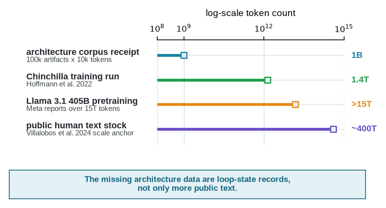
To see why we cannot simply extract this state from internet-scale text, the token count makes the contrast sharper. A broad corpus of public computer-architecture knowledge is only on the order of \(10^9\) tokens. The architecture-relevant subset of the Wikipedia corpus sits at that scale, and a back-of-the-envelope cross-check from roughly fifty years of the literature agrees, at about 100,000 papers of 10,000 tokens each: \[ T_{\mathrm{arch\text{-}text}} \approx N_{\mathrm{artifacts}} \times \bar{t}_{\mathrm{artifact}} \approx 10^5 \times 10^4 \approx 10^9 \ \mathrm{tokens}. \] That sounds large, but it is small by web-scale pretraining standards. More importantly, it is incomplete in the wrong way. Papers preserve accepted claims far better than failed configurations, simulator flags, workload revisions, EDA reports, review arguments, and rejected alternatives. Architecture 2.0 therefore cannot treat “all architecture text” as the dataset. The dataset must include the loop state that made the text credible, and it must expose enough tacit judgment to make assumptions, exclusions, and rejection decisions inspectable. The token count matters only because it limits what a generative method can infer about action authority. Text may retrieve concepts, but it cannot recover which candidate was legal, what feedback was observed, why alternatives were rejected, or who accepted the risk.
Pretraining: The computationally intensive initial phase of training a large machine learning model on a massive, general dataset before fine-tuning it for specific tasks.
Both are order-of-magnitude anchors, not a measured corpus inventory. The transparent literature calculation and the architecture-relevant Wikipedia corpus land at the same \(10^9\)-token scale. Table 4.3 shows why the exact token count is not the main claim. The important scarcity is that the most useful architecture data are often not public, not textual, or not preserved as reusable loop state.
| Data layer | Rough public visibility | What is missing for Architecture 2.0 |
|---|---|---|
| Published papers, manuals, and tutorials | Public and mostly textual. | Failed runs, rejected alternatives, exact workload slices, scripts, seeds, and review rationale. |
| Open-source RTL, simulators, compilers, and benchmarks | Public but heterogeneous and version-sensitive. | Tool settings, run provenance, invalid configurations, and cross-tool disagreement. |
| Commercial EDA reports, PDK assumptions, and signoff context | Often private or redacted. | Timing, power, physical, waiver, and closure evidence tied to the claim. |
| Design reviews and engineer memory | Usually tacit. | Why an experiment was abandoned, which proxy was distrusted, and who accepted risk. |
To visualize just how small the public-text estimate is, Figure 4.1 puts the architecture token count on the same log-scale axis as three public AI-data anchors: the 1.4 trillion tokens used to train DeepMind’s Chinchilla model, Meta’s report that Llama 3.1 405B was trained on more than 15 trillion tokens, and a public human-text-stock estimate on the order of hundreds of trillions of tokens (Hoffmann et al. 2022; Meta AI 2024; Villalobos et al. 2024). The point is not that architecture should race to scrape the web. The point is that even a generous public architecture-text estimate is tiny by modern pretraining standards, while the most important missing records are not ordinary text at all.
Hoffmann, Jordan, Sebastian Borgeaud, Arthur Mensch, et al. 2022. “Training Compute-Optimal Large Language Models.” Advances in Neural Information Processing Systems 35: 30016–30. https://doi.org/10.48550/arXiv.2203.15556.
Meta AI. 2024. Introducing Llama 3.1: Our Most Capable Models to Date. https://ai.meta.com/blog/meta-llama-3-1/.
Villalobos, Pablo, Anson Ho, Jaime Sevilla, Tamay Besiroglu, Lennart Heim, and Marius Hobbhahn. 2024. Will We Run Out of Data? Limits of LLM Scaling Based on Human-Generated Data. https://doi.org/10.48550/arXiv.2211.04325.
Table 4.4 makes the receipt explicit. It is not a measured corpus inventory. It is a scale check that separates the easy counts from the hard missing records. The multiplication that gives \(10^9\) tokens is deliberately simple; the point is that even a generous public-text corpus is small, and the public surfaces we can count most easily are not the same thing as architecture loop state. Treat the counts themselves as a release-time snapshot, not a durable benchmark.
| Receipt | Current value | What it supports | Caveat |
|---|---|---|---|
| Public architecture, systems, and EDA artifacts | \(10^5\) paper-equivalent artifacts | Order-of-magnitude basis for the \(10^9\)-token scale check. | Assumption for intuition; not a measured corpus boundary. |
| Tokens per paper-equivalent artifact | \(10^4\) tokens per artifact | Transparent multiplication: \(10^5 \times 10^4 = 10^9\). | Tokenization and artifact length vary; manuals and specifications can be much larger. |
| DBLP title pilot | 1,015 title records from selected ISCA, MICRO, HPCA, and ASPLOS years | Shows that public metadata is easy to collect and useful for trajectory signals. | Title-only pilot; not full text, artifacts, tool state, or design-loop evidence. |
| GitHub RTL language proxy | 141,288 Verilog repositories; 43,371 SystemVerilog repositories | Shows a large public RTL-adjacent surface that could seed artifact mining. | Broad language counts include small, toy, forked, stale, and non-architecture repositories. |
| GitHub RTL keyword proxy | 4,292 Verilog+“rtl” repositories; 1,657 SystemVerilog+“rtl” repositories | Gives a narrower proxy for RTL-oriented repositories. | Keyword-sensitive and unvalidated; it is still not a count of usable architecture design examples. |
| GitHub topic proxy | 353 computer-architecture-tagged Verilog repositories; 1,817 FPGA-tagged Verilog repositories | Shows that curated labels are much smaller than broad language counts. | Topic labels are voluntary, incomplete, and uneven across projects. |
| Missing loop-state records | Not counted | The highest-value architecture data are traces, configs, logs, reports, reviews, negative results, and rejected candidates. | Much of this state is private, tacit, uncodified, or discarded before publication. |
The useful lesson from the receipt is the mismatch. A title corpus can help map topic drift, but it cannot recover simulator flags, failed configurations, or review arguments. A Verilog repository count can show that public RTL-like material exists, but it does not say whether the repository contains a well-specified architecture decision, a reusable testbench, a valid workload, or evidence that rejected alternatives were considered. Architecture 2.0 therefore needs corpus building only when artifacts are converted into loop records: candidate, workload, tool version, legal and invalid actions, feedback, provenance, rejected alternatives, and decision owner.
Domain adaptation matters here only if it helps construct or retrieve loop records; vocabulary and retrieval gains do not grant an automated optimizer action authority. The medical AI lineage is a useful comparison because it shows both the power and the limit of domain adaptation. BioBERT adapted a general language model to biomedical text; ClinicalBERT adapted representations to clinical notes; Med-BERT adapted BERT-style pretraining to structured electronic health records rather than ordinary prose (Lee et al. 2020; Huang et al. 2019; Rasmy et al. 2021). Those systems mattered because they treated the domain’s data format as a first-order problem. Chip design has its own instance. ChipNeMo adapts language models to hardware-design text with a custom tokenizer, domain-continued pretraining, and retrieval over internal corpora, then applies them to engineering question-answering, electronic-design-automation script drafting, and bug-report summarization (Liu et al. 2023). It demonstrates that domain adaptation can improve text-facing hardware tasks, and it illustrates the limit this chapter presses. It maps text to text, so it addresses the data-ingestion problem, not action authority in a closed design loop. Architecture must do the same domain work, but the representation burden is broader. A compute-subsystem design loop needs not only domain terms, but also executable tool state, workload provenance, constraints, multi-fidelity feedback, rejected alternatives, and decision authority. A paper corpus can bootstrap knowledge; it cannot by itself represent the design loop.
Lee, Jinhyuk, Wonjin Yoon, Sungdong Kim, et al. 2020. “BioBERT: A Pre-Trained Biomedical Language Representation Model for Biomedical Text Mining.” Bioinformatics 36 (4): 1234–40. https://doi.org/10.1093/bioinformatics/btz682.
Huang, Kexin, Jaan Altosaar, and Rajesh Ranganath. 2019. “ClinicalBERT: Modeling Clinical Notes and Predicting Hospital Readmission.” arXiv Preprint arXiv:1904.05342. https://arxiv.org/abs/1904.05342.
Rasmy, Laila, Yang Xiang, Ziqian Xie, Cui Tao, and Degui Zhi. 2021. “Med-BERT: Pretrained Contextualized Embeddings on Large-Scale Structured Electronic Health Records for Disease Prediction.” Npj Digital Medicine 4 (86). https://doi.org/10.1038/s41746-021-00455-y.
Liu, Mingjie, Teodor-Dumitru Ene, Robert Kirby, et al. 2023. ChipNeMo: Domain-Adapted LLMs for Chip Design. arXiv preprint arXiv:2311.00176. https://arxiv.org/abs/2311.00176.
Domain adaptation: A machine learning technique where a model trained on one data distribution is adjusted to perform well on a different, specific target domain (Pan and Yang 2010).
Pan, Sinno Jialin, and Qiang Yang. 2010. “A Survey on Transfer Learning.” IEEE Transactions on Knowledge and Data Engineering 22 (10): 1345–59. https://doi.org/10.1109/TKDE.2009.191.
Domain-continued pretraining: Further training a foundational model on a large corpus of domain-specific text to improve its specialized vocabulary and understanding.
Moving from training text to evaluation, benchmark lineages such as SQuAD and GLUE offer a related lesson. Shared, scoreable examples can move a whole field. The Architecture 2.0 lesson is not to seek a cheap labeled row, but to ask what a shared evaluation object must record before an automated optimizer can act. Architecture needs shared evaluation objects too, but their purpose is not only scoring models; it is constraining what an automated optimizer may try next, what evidence can update the loop, and what a human reviewer can reject. An architecture “example” is rarely just a cheap labeled row. It may be a simulator run, a synthesis run, a physical-design report, a workload trace, a failed configuration, or an expert review tied to a specific fidelity level. The cost of a sample is therefore part of the representation problem, not an afterthought.
SQuAD and GLUE: Standard benchmark datasets used to evaluate the performance of natural language processing models, where SQuAD is the Stanford Question Answering Dataset (Rajpurkar et al. 2016) and GLUE is the General Language Understanding Evaluation (Wang et al. 2018).
Rajpurkar, Pranav, Jian Zhang, Konstantin Lopyrev, and Percy Liang. 2016. “SQuAD: 100,000+ Questions for Machine Comprehension of Text.” Proceedings of the 2016 Conference on Empirical Methods in Natural Language Processing, 2383–92. https://doi.org/10.18653/v1/D16-1264.
Wang, Alex, Amanpreet Singh, Julian Michael, Felix Hill, Omer Levy, and Samuel R. Bowman. 2018. “GLUE: A Multi-Task Benchmark and Analysis Platform for Natural Language Understanding.” Proceedings of the 2018 EMNLP Workshop BlackboxNLP: Analyzing and Interpreting Neural Networks for NLP, 353–55. https://doi.org/10.18653/v1/W18-5446.
4.2 Sample Cost Is Architecture Data
Because this cost dictates how an optimizer must treat an evaluation point, we have to move away from the web-centric view of a sample. In many benchmark settings, a sample is treated merely as an input-output pair: a question and answer, an image and label, a prompt and reference response. In an architecture design loop, a sample is better understood as a feedback event that changes what the loop believes. It might be a cycle-level simulation, a compiler report, a failed synthesis run, a power estimate, a rejected floorplan, an expert review, or a silicon measurement. Each event has a cost, fidelity, provenance, and commitment level.
Architecture sample. An architecture sample is any feedback event that changes the loop’s belief about a design candidate, including its cost, fidelity, provenance, assumptions, rejected-space coverage, and commitment level.
For an automated design loop, sample cost is part of the action policy. It determines which evaluations are cheap enough to explore, which require escalation, and which decisions should remain human-owned.
Architect’s checkpoint: The Cost of Fidelity
Before the loop consumes days of compute on a cycle-accurate simulation or physical synthesis run, it must hit a fidelity gate. The architect must own the decision to authorize expensive, high-fidelity samples, balancing the exploration budget against the cost of the feedback event.
A useful representation should therefore record the burden and evidence context of feedback, not only the feedback value. A sample is best written as a vector of incommensurable dimensions, not a single number, since they do not share units: \[ \begin{aligned} M_{\mathrm{sample}} = \langle\, & C_{\mathrm{setup}}, C_{\mathrm{tool}}, C_{\mathrm{license}}, C_{\mathrm{compute}}, C_{\mathrm{human}}, \\ & F_{\mathrm{fidelity}}, P_{\mathrm{provenance}}, K_{\mathrm{coverage}}, C_{\mathrm{opportunity}}, C_{\mathrm{risk}} \,\rangle . \end{aligned} \]
The vector does not collapse into one currency; its dimensions carry different units. It is a reminder that an architecture sample carries hidden state. A simulator point may require setup time, tool availability, license access, calibration work, human triage, provenance, coverage context, and the opportunity cost of not evaluating another candidate. A post-layout result may carry higher fidelity but also higher latency and risk. A field deployment measurement may be authoritative for one population and irrelevant for another.
Concrete architecture tools span this range. Analytical mapping and dataflow models are designed for broad design-space exploration (Parashar et al. 2019; Kwon et al. 2019). Physical-design and verification flows expose the other end of the spectrum, where feedback can take hours or days and the human and engineering cost becomes part of the sample itself (Mirhoseini et al. 2021; Semiconductor Industry Association 2026; Bauer et al. 2020; Foster 2022). Table 4.5 is therefore not a tool taxonomy. It is a representation checklist. If the row changes, the loop must record different state.
Parashar, Angshuman, Priyanka Raina, Yakun Sophia Shao, et al. 2019. “Timeloop: A Systematic Approach to DNN Accelerator Evaluation.” 2019 IEEE International Symposium on Performance Analysis of Systems and Software, ISPASS, 304–15. https://doi.org/10.1109/ISPASS.2019.00042.
Kwon, Hyoukjun, Prasanth Chatarasi, Michael Pellauer, Angshuman Parashar, Vivek Sarkar, and Tushar Krishna. 2019. “Understanding Reuse, Performance, and Hardware Cost of DNN Dataflows: A Data-Centric Approach.” Proceedings of the 52nd Annual IEEE/ACM International Symposium on Microarchitecture, MICRO ’52, 754–68. https://doi.org/10.1145/3352460.3358252.
Semiconductor Industry Association. 2026. Chip Design and R&D. https://www.semiconductors.org/policies/chip-design/.
Bauer, Harald, Ondrej Burkacky, Peter Kenevan, Stephanie Lingemann, Klaus Pototzky, and Bill Wiseman. 2020. Semiconductor Design and Manufacturing: Achieving Leading-Edge Capabilities. McKinsey & Company report. https://www.mckinsey.com/industries/semiconductors/our-insights/semiconductor-design-and-manufacturing-achieving-leading-edge-capabilities.
Foster, Harry. 2022. Part 8: The 2022 Wilson Research Group Functional Verification Study. Verification Horizons, Siemens EDA. https://blogs.sw.siemens.com/verificationhorizons/2022/12/12/part-8-the-2022-wilson-research-group-functional-verification-study/.
| Feedback source | Latency / cost intuition | What it exposes | Record for reuse |
|---|---|---|---|
| Analytical model or mapper | Milliseconds to seconds; low direct cost; high model-risk exposure. | Useful for pruning and sensitivity checks, not final evidence. | Model assumptions, workload slice, constraints, and proxy-validity notes. |
| Trace, profile, or replay | Seconds to hours depending on capture and replay setup. | Workload provenance is part of the sample. | Trace version, sampling policy, software stack, and filtering choices. |
| Cycle-level simulation | Minutes to days depending on model detail and target workload. | Simulator evidence is scoped by abstraction, calibration, and unsupported states. | Simulator version, configuration, seeds, workload revision, and calibration notes. |
| RTL, gate, or EDA feedback | Hours to days when synthesis, timing closure, power analysis, or physical DRC/LVS feedback enters the loop. | High-fidelity samples are scarce and multiobjective. | Tool versions, constraints, process assumptions, waived warnings, and rejected candidates. |
| FPGA, emulation, or prototype | High setup and shared-resource cost; high throughput once mapped. | Speed changes observability and debugging semantics, not only wall-clock time. | Mapping constraints, observability limits, debug hooks, and queue/resource state. |
| Silicon or field telemetry | Weeks to years and high commitment. | Authoritative measurements still require context and human decision authority. | Population, deployment version, rollback policy, incident context, and decision owner. |
For tools like simulators, the timing side of this cost is multiplicative. A simulator is not slow in the abstract; it is slow relative to the target cycles the workload demands. For a target clock \(f_{\mathrm{target}}\), workload duration \(T_{\mathrm{workload}}\), and simulation throughput \(R_{\mathrm{sim}}\), the wall time is \[ T_{\mathrm{wall}} = \frac{N_{\mathrm{cycles}}}{R_{\mathrm{sim}}} = \frac{f_{\mathrm{target}} \times T_{\mathrm{workload}}}{R_{\mathrm{sim}}}. \] Table 4.6 gives the intuition for a 1 GHz target. Read each row as a span of target execution time, each column as a simulator throughput, and each cell as the wall-clock time to simulate that span. One second of a 1 GHz target takes about 11.6 days at 1 kcycle/s but only 10 s at 100 Mcycle/s. The rates are illustrative, but the multiplication is the point. A loop can afford many cheap proxy samples, fewer cycle-level samples, and very few high-fidelity samples unless it has a disciplined plan for escalation and rejection.
| Target workload at 1 GHz | Target cycles | 1 kcycle/s | 100 kcycle/s | 10 Mcycle/s | 100 Mcycle/s |
|---|---|---|---|---|---|
| 1 ms | \(10^{6}\) | 16.7 min | 10 s | 0.1 s | 0.01 s |
| 1 s | \(10^{9}\) | 11.6 days | 2.8 h | 1.7 min | 10 s |
| 1 min | \(6\times 10^{10}\) | 1.9 years | 6.9 days | 1.7 h | 10 min |
| 1 h | \(3.6\times 10^{12}\) | 114 years | 1.1 years | 4.2 days | 10 h |
This cost structure changes how we should think about design spaces. A small co-design exercise with five workload slices, four architecture configurations, and six compiler or mapping settings has \(5 \times 4 \times 6 = 120\) candidates and can sometimes be enumerated. A physical-design, compiler, mapping, or chiplet-integration space may be combinatorial, sequential, tool-bound, and partially invalid. Learning-assisted chip placement makes the point concrete. The design problem can be formulated as a learning problem, but the value of each sample depends on the representation of macros, nets, constraints, tool feedback, and placement validity (Mirhoseini et al. 2021); that result was later contested on its baselines and reproducibility (Chapter 7) (Cheng, Kahng, and others 2023), which only sharpens the point. The architecture lesson is broader than placement. When samples are expensive, the loop record must capture what each sample cost, what region of the space it informs, what it rules out, and how it should constrain the next optimizer action.
Cheng, Chung-Kuan, Andrew B. Kahng, et al. 2023. “Assessment of Reinforcement Learning for Macro Placement.” Proceedings of the 2023 International Symposium on Physical Design (ISPD). https://doi.org/10.1145/3569052.3578926.
Chapter 6 returns to sample efficiency from the method side. The representation lesson comes first. If cost, fidelity, and rejected-space coverage are not recorded, a later optimizer cannot know whether it is learning the design space or merely collecting disconnected measurements.
4.3 Architecture Descriptions as Boundary Objects
All of that recorded state has to live somewhere the loop and the architect can both read, and that artifact, the architecture description, is a boundary object. In the sense introduced by Star and Griesemer, a boundary object is shared across communities while still supporting their different local uses (Star and Griesemer 1989). It sits between human intent and tool action. It must be readable enough for architects to inspect, precise enough for tools to execute, and structured enough for automated optimizers or methods to modify without breaking the design contract.
Star, Susan Leigh, and James R. Griesemer. 1989. “Institutional Ecology, ‘Translations’ and Boundary Objects: Amateurs and Professionals in Berkeley’s Museum of Vertebrate Zoology, 1907–39.” Social Studies of Science 19 (3): 387–420. https://doi.org/10.1177/030631289019003001.
At minimum, an architecture description should make the action contract explicit: what is being described, what can change, what must not change, what evidence can update the record, and which tools can consume it. For a memory hierarchy, this may include cache sizes, associativity, replacement policy, prefetching, coherence assumptions, bandwidth, latency, and workload mix. For an accelerator or compute subsystem, it may include supported operations, data layout, local storage, vector width, dataflow, quantization, compiler/runtime assumptions, and fallback behavior. For an optimizer-facing architecture description, the minimum is not only fields but permissions: which fields are mutable, which are read-only constraints, which tool observations can update them, and which violations trigger rejection or escalation.
The important point is not that every representation must be one universal schema. Different loops need different representations. A paper-reading loop, a simulator-driven design-space exploration loop, an RTL-generation loop, and a post-silicon telemetry loop should not have identical records. But they do need explicit invariants. What fields must be present? Which fields can a method change? Which fields are read-only constraints? Which assumptions travel with a result? Which tool versions, seeds, and workload revisions are required for replay?
Without those boundaries, a representation becomes a prompt-shaped anecdote. It may sound plausible, but it cannot safely drive action.
4.4 Unstructured Design Data and Its Cost
When those boundaries are left implicit, the missing structure does not stay free. Architecture teams accumulate undocumented design state, the same kind of hidden cost that software teams call technical debt when complex data dependencies and implicit assumptions go unmanaged (Sculley et al. 2015). The cost appears whenever important design state exists but is not captured in a durable, inspectable form. It may live in shell scripts, simulator flags, spreadsheet formulas, plotting notebooks, benchmark directories, issue threads, email, review slides, or the memory of the person who knows why one candidate was rejected. Some of this state is tacit rather than textual: what an experienced architect chooses not to try, which proxy result they distrust, which corner case they ask about in review, and which risk they refuse to delegate.
Sculley, David, Gary Holt, Daniel Golovin, et al. 2015. “Hidden Technical Debt in Machine Learning Systems.” Advances in Neural Information Processing Systems 28.
Mirhoseini, Azalia, Anna Goldie, Mustafa Yazgan, et al. 2021. “A Graph Placement Methodology for Fast Chip Design.” Nature 594 (7862): 207–12. https://doi.org/10.1038/s41586-021-03544-w.
Cheng, Chung-Kuan, Andrew B. Kahng, Sayak Kundu, Yucheng Wang, and Zhiang Wang. 2023. “Assessment of Reinforcement Learning for Macro Placement.” Proceedings of the 2023 International Symposium on Physical Design (ISPD). https://doi.org/10.1145/3569052.3578926.
Markov, Igor L. 2023. “The False Dawn: Reevaluating Google’s Reinforcement Learning for Chip Macro Placement.” arXiv Preprint arXiv:2306.09633.
Goldie, Anna, Azalia Mirhoseini, Amir Yazdanbakhsh, and Jeff Dean. 2024. “That Chip Has Sailed: A Critique of Unfounded Skepticism Around AI for Chip Design.” arXiv Preprint arXiv:2411.10053.
This gap is manageable when a small team manually coordinates the loop. It becomes a technical failure when an AI system acts inside the loop. If a constraint is implicit, the method may violate it. If a simulator flag is hidden, the result may not be replayable. If rejected candidates are missing, the search may rediscover known failures. If workload provenance is unclear, the loop may optimize for the wrong distribution. If plots preserve only the winning candidate, the evidence trail cannot explain why alternatives were discarded. ::: {.callout-field-note title=“The result no one could rerun”} Consider AI-generated chip placement. A reinforcement-learning method was reported to place macros as well as or better than human experts, and said to have run on production silicon (Mirhoseini et al. 2021); independent groups then could not reproduce the advantage, because the code and pretraining inputs needed to rerun it were never released (Cheng, Kahng, Kundu, et al. 2023; Markov 2023), and the authors answered that the critics had not run the method as described (Goldie et al. 2024). Years later the claim can be neither confirmed nor rejected. The lesson is not who is right; it is that a result no one can rerun leaves the loop with an anecdote instead of evidence.
Takeaway. Enforce tool and environment provenance as the run happens, so the loop leaves a replayable receipt rather than a dispute. ::: To show where this missing information typically hides, Table 4.7 gives common sources of undocumented design state. The point is not to document everything for its own sake. The point is to capture enough state that a loop can compare, replay, reject, and revise.
| Artifact | What it enables | What it often hides | Failure mode |
|---|---|---|---|
| Paper or plot | Claim, result, and comparison. | Tool flags, failed candidates, tuning history. | Reproduce only the story, not the loop. |
| Workload trace | Concrete input behavior and measurements. | Coverage, versioning, sampling policy, privacy filters. | Optimize for an unrepresentative slice. |
| Simulator config | Replayable model setting. | Defaults, unsupported states, calibration limits. | Trust a number outside its valid scope. |
| RTL or EDA report | Implementation-facing feedback. | Process assumptions, constraints, waived warnings. | Accept an artifact that cannot close. |
| Review notes | Human judgment and rationale. | Tacit assumptions and discarded alternatives. | Lose why a decision was made. |
| Rejected candidate | Search boundary and negative evidence. | Why it failed and at what fidelity. | Rediscover known dead ends. |
4.5 QuArch as a Stress Test
The artifacts in Table 4.7 are internal and often unstructured. Public benchmarks sit at the opposite extreme, well structured but paper-bound. QuArch, a question-answering benchmark that turns the architecture literature into a structured, expert-validated evaluation object (Prakash et al. 2025b), is a useful stress test for this chapter precisely because it exposes what that public structure still leaves out. It bridges two representation layers, architecture knowledge that can be asked about in text and architecture state that must be carried by a loop before an automated optimizer can act. The later QuArch reasoning benchmark makes the same point more explicit by organizing 2,671 expert-validated questions around recall, analysis, design, and implementation competencies (Prakash et al. 2025a). QuArch can ask whether a model recalls concepts, tracks architectural relationships, reasons over published claims, and avoids obvious domain mistakes. That is valuable. A field cannot build credible AI-assisted systems if those systems lack basic architectural knowledge.
Prakash, Shvetank et al. 2025b. “QuArch: A Question-Answering Dataset for AI Agents in Computer Architecture.” IEEE Computer Architecture Letters, ahead of print. https://doi.org/10.1109/LCA.2025.3541961.
Prakash, Shvetank et al. 2025a. QuArch: A Benchmark for Evaluating LLM Reasoning in Computer Architecture. https://arxiv.org/abs/2510.22087.
Figure 4.2 shows why that achievement is necessary but not sufficient. Paper-derived questions test one layer of architecture data, while action and rejection require loop-state records that papers often omit.
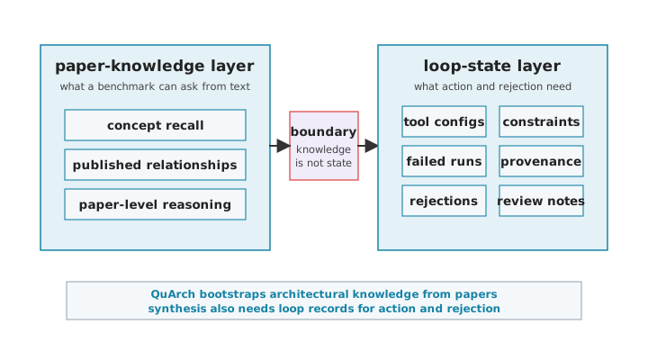
As this boundary test highlights, the limit of paper-derived datasets like QuArch is that papers preserve accepted claims far better than they preserve design-loop state. They rarely contain every simulator configuration, rejected candidate, failed run, hidden constraint, calibration choice, or review argument. A model that answers questions over papers may know what a concept means and still lack the state needed to act inside a design loop. It may summarize a memory-system paper, but it does not necessarily know which candidates failed, which simulator flags were decisive, which workload slices were excluded, or which result would cause a human architect to reject the next proposal.
The lesson is not that question-answering datasets are insufficient and therefore unimportant. The lesson is that they occupy one layer. They help represent architectural knowledge. Architecture 2.0 also needs representations of experiments, tools, constraints, provenance, and negative traces. A reader should see QuArch as one example of bootstrapping the data layer, not as the whole data layer.
4.6 Toward Architecture World Models
If the data layer described above—including both paper-derived knowledge and loop-state records—constitutes the representation, the loop still needs a mechanism to act on it. Representation records what the loop knows; the world model, the second half of the pairing, is what turns that record into predicted consequences. The world-model idea becomes architecture-specific when it is tied to tool behavior, cost, constraints, invalid-action rules, uncertainty, and decision policies, much like reinforcement learning agents use latent world models2 to plan and simulate outcomes before acting.
2 Internal, compressed representations of an environment used by an AI to simulate and plan actions without interacting with the real world.
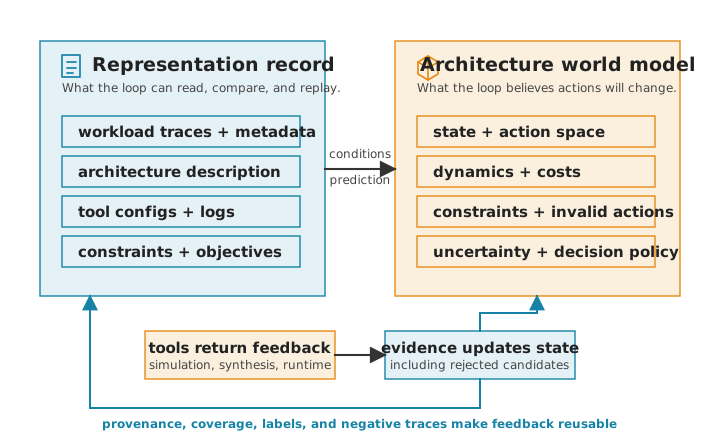
This distinction matters. A simulator configuration is part of the representation. The simulator’s behavior, scope, calibration, and failure modes are part of the world model. A table of candidate parameters is representation. A surrogate that predicts latency or energy from those parameters is a world model. A set of design rules, expert heuristics, or physical constraints can also act as a world model.
Figure 4.3 gives the basic structure. A representation record contains workload traces, architecture descriptions, tool configurations, logs, constraints, and objectives. A world model contains state, action spaces, dynamics, costs, constraints, invalid-action rules, uncertainty, and decision policies. Tools return feedback; evidence updates both the representation and the world model.
For the lighthouse prompt, a small world model might be as simple as Table 4.8. It is not a full simulator. It is the part of the loop’s belief that says which actions are meaningful, what they are expected to change, and what evidence can overturn the prediction.
| World-model field | XRBench/RISC-V sketch |
|---|---|
| State | Workload slice, frame deadline, software path, candidate compute organization, memory traffic, and power envelope. |
| Legal action | Change vector width, local memory size, CPU/accelerator partition, or data layout inside the declared software contract. |
| Predicted transition | Estimate latency, memory traffic, energy, area pressure, and compiler/runtime feasibility. |
| Uncertainty and calibration | State whether the estimate comes from an analytic proxy, calibrated simulator, prior measurements, or expert rule. |
| Invalid-action rule | Reject candidates that break software compatibility, exceed the action bounds, fail correctness, or lack provenance. |
| Escalation trigger | Move to stronger evidence when a candidate nears the 3 W target, misses the frame deadline, or wins only under a weak proxy. |
The type of world model matters only through the loop contract it supports: what actions it can evaluate, what uncertainty it reports, what invalid moves it rejects, when it escalates fidelity, and which decisions remain human-owned. A simulator-backed world model uses a tool as the transition and feedback mechanism. A learned surrogate world model predicts outcomes from prior evaluations. A symbolic or constraint-based world model encodes invalid configurations, design rules, or physical limits. A hybrid world model combines these pieces: a simulator for selected candidates, a learned predictor for cheap screening, a rule system for invalid actions, and an escalation rule that routes high-commitment decisions out to human review.
No world model is automatically credible. Each has a scope. Each has uncertainty. Each can be wrong under distribution shift, new workloads, different software stacks, tool changes, or higher-fidelity evaluation. The goal is not to pretend the world model is truth. The goal is to make its assumptions explicit enough that the loop can decide when to trust it, when to escalate fidelity, and when to reject its advice. The lighthouse prompt makes that discipline concrete. An analytic proxy predicts that a wider-vector candidate meets the 3 W envelope, but the margin to the envelope is smaller than the proxy’s known error band, so the escalation trigger from Table 4.8 fires. A calibrated simulator then shows the candidate misses the frame deadline on the real XRBench slice, and the architect records the rejection with its fidelity level and reason. The prediction, the escalation, and the rejection are all part of the world model, and each is auditable. An automated optimizer acted on the belief, and a human could see why it was overturned.
Distribution shift: A situation where the data a model encounters during deployment differs significantly from the data it was trained on, often degrading performance (Quinonero-Candela et al. 2009).
Quinonero-Candela, Joaquin, Masashi Sugiyama, Anton Schwaighofer, and Neil D. Lawrence, eds. 2009. Dataset Shift in Machine Learning. MIT Press.
Architect’s checkpoint: Escalate or Reject
When the world model proposes a candidate whose margin of safety is smaller than the model’s known error band, the loop must pause. The architect decides whether to escalate to a higher-fidelity tool (e.g., a cycle-level simulator) or reject the candidate outright based on risk. This gate ensures the optimizer does not commit to decisions based on uncalibrated proxy estimates.
4.7 Provenance, Coverage, and Negative Traces
Knowing when to reject the world model’s advice depends on records most teams are quick to discard. The most distinctive architecture data may be the data the field usually throws away. Published work tends to preserve accepted artifacts. Design loops also need rejected alternatives. A failed simulator run, invalid configuration, proxy win that fails at higher fidelity, abandoned floorplan, or unsupported-software path is not merely noise. It shows the loop where the boundary lies.
Venues for negative results: The wider computing-systems community has begun to build places to publish exactly these records, such as the NOPE workshop (Negative results, Opportunities, Perspectives, and Experiences) held with ASPLOS. The field needs more of them, so that failed runs, rejected candidates, and the assumptions behind them accumulate as shared evidence instead of being discarded before publication.
Negative traces. Negative traces are recorded failed, rejected, invalid, or abandoned candidates together with the reason they did not support the claim. They matter because a loop that records only winners cannot inform the next method, reviewer, or architect which assumptions, tools, workloads, or regions of the design space were already ruled out.
Negative traces matter because architecture action spaces are full of invalid or misleading moves. A generated RTL fragment may be syntactically plausible but fail timing or violate an interface. A design-space search may find a candidate that looks good under a proxy but fails under a better power model. A benchmark result may improve because the workload slice is too narrow. A chiplet partition may appear modular but introduce unacceptable latency, thermal coupling, test complexity, or supply-chain risk.
Table 4.9 turns this point into a data schema. The purpose is to record what failed, what boundary it exposed, and how that evidence should change the next action in the loop.
| Negative trace | What it records | What the loop learns |
|---|---|---|
| Synthesis or timing violation | Constraints, process, parameters, failing setup/hold paths. | Exclude this macro or parameter combination. |
| Unroutable or PDN failing netlist | Placement, density, pin layout, congestion map, IR drop. | Add congestion-aware spacing or reshape the action space. |
| Proxy win that fails fidelity | Cheap metric improves, but stronger evaluation rejects it. | Calibrate proxies and require sensitivity checks. |
| Tool failure or crash | Simulator, synthesis, compiler, or harness cannot complete. | Separate design failure from environment failure. |
| Coverage gap | Workload, input, scenario, or architecture class was not represented. | Mark the evidence boundary before committing. |
| Rejected design rationale | Human review rejects a candidate for risk, maintainability, schedule, or integration. | Preserve architect judgment as training and audit data. |
Negative traces require provenance—an exact, replayable record of the environment that produced the result. A failed result without context is not very useful. The minimum reusable record includes the candidate identifier, workload slice, software stack, tool version, seed, parameters, constraints, fidelity level, failure reason, coverage boundary, and decision owner. The loop also needs coverage. What part of the design space, workload space, or evidence regime does this trace represent? Without provenance and coverage, negative traces become a pile of anecdotes. With them, they become architecture data.
4.8 When a Representation Becomes Actionable
Collecting this architecture data—from high-fidelity negative traces to structured constraints and world-model escalation triggers—ultimately serves a single goal, enabling automation. A representation becomes actionable when it can safely support loop operations. It should define valid actions, expose relevant observations, carry constraints and objectives, record provenance, support replay, preserve uncertainty, separate feedback from evidence, and record what rejects a candidate. It should also say what remains a human decision.
This is a higher bar than asking whether a model can read it. A representation that can be summarized may still be useless for design. A representation that can be searched may still hide invalid actions. A representation that produces a score may still lack provenance. A representation that captures winning results but not rejected alternatives may give the loop a biased view of the space.
The same test applies to abstractions. A useful Architecture 2.0 abstraction does not merely hide detail or provide nicer names. It creates a surface where valid actions, feedback, rejection, replay, or review can happen earlier, cheaper, or with clearer authority. An abstraction that cannot return feedback is merely notation; it may help people talk, but it has not yet made the loop more capable.
For the lighthouse prompt, an actionable representation would not merely contain the prompt text. It would include the XRBench scenario, workload metadata, architecture parameters, software assumptions, power and process constraints, tool configurations, candidate set, feedback budget, evidence regime, negative traces, and rejection authority. Only then can the loop ask a bounded question: which candidate should be evaluated next, which evidence is strong enough, and which decision still belongs to the architect?
Design principle: Make architecture work legible to the automated loop
A representation earns trust only when it records provenance, assumptions, costs, failures, and negative traces, not only the successful endpoints. What the loop cannot see, it cannot reason about, and what the human architect cannot see, they cannot safely reject.
4.9 Conclusion
This chapter asked what architecture data must record before an automated optimizer can act on it and a human architect can audit the result. Representation is the first hard problem because a method can only act on what the loop can see. Get it wrong and a more capable model simply moves faster in the wrong direction. Get it right and the loop gains a surface where valid actions, feedback, rejection, replay, and review can actually happen.
Legibility is the bar, and it sits higher than readability. A representation is actionable only when it defines valid actions, exposes relevant observations, carries constraints and objectives, records provenance, supports replay, preserves uncertainty, separates feedback from evidence, records what can reject a candidate, and says what remains a human decision. A representation that captures winning results but not rejected alternatives, or scores but not provenance, hands the loop a biased and unauditable view of the space.
The durable rule is to make architecture work legible to the automated loop, which means recording provenance, assumptions, costs, failures, and negative traces, not only the successful endpoints. What the loop cannot see, it cannot reason about, and what the architect cannot see, they cannot safely reject. World models, structured design data, and negative-trace corpora all serve that one end, turning scattered architecture experience into state a loop can read, replay, compare, and revise.
4.10 Open Research Questions
As we have seen, the gap between public architecture knowledge and actionable loop state is significant. This gap leaves several unsettled research directions for the community to explore. Solving these requires moving beyond static data to dynamic, fidelity-aware representations that can safely guide an automated optimizer.
What is the formal semantics of an auditable architecture proposal? While representations must act as boundary objects between human intent and tool execution (see the discussion on “Architecture Descriptions as Boundary Objects” in Section 4.3), we lack a rigorous calculus for optimizer proposals. A thesis-level challenge is to define a canonical, machine-readable schema for loop-state records that supports independent replay, checking, and safe rejection of an AI-generated architecture candidate using its attached provenance.
Can world models discover and navigate fidelity frontiers? Building on the escalation triggers defined in our world model sketch (Table 4.8), future research must move beyond static rule-based thresholds. An open challenge is to develop predictive surrogates that learn their own calibration boundaries and route high-risk design evaluations to cycle-accurate simulation or physical synthesis when the loop’s evidence boundary is exceeded, thereby managing the trade-off between sample cost and prediction risk.
What is the information-theoretic limit of generalization in AI-driven design? As emphasized by treating sample cost as architecture data (see the discussion on “Sample Cost Is Architecture Data” in Section 4.2), workload provenance is critical loop state. Yet, we lack rigorous methods to detect when an automated optimizer has overfit to a specific execution phase or synthetic input distribution. A major research direction is establishing formal generalization bounds3 for architecture agents, helping prevent silent hardware failures under distribution shifts toward architecture world models (see the discussion on “Toward Architecture World Models” in Section 4.6).
How do we formulate representation learning over negative architecture traces? As established in our discussion of provenance, coverage, and negative traces (see the discussion on “Provenance, Coverage, and Negative Traces” in Section 4.7), rejected candidates, missed timing constraints, and invalid parameters define the true boundary of the design space (Table 4.9). However, current generative models are primarily trained on successful artifacts. A critical problem for the ML-for-systems community is designing novel loss functions4 or preference-optimization pipelines5 that force models to learn from high-fidelity negative records, ensuring they actively avoid—rather than rediscover—known failure modes.
3 Theoretical limits on how well a machine learning model’s performance on its training data will apply to unseen, out-of-distribution data.
4 Mathematical functions used to measure the difference between an AI model’s predicted output and the actual target, which the training process seeks to minimize.
5 Techniques like Reinforcement Learning from Human Feedback (RLHF) or Direct Preference Optimization (DPO) used to align a model’s outputs with human preferences.
What to carry forward
- Reader test: Could an automated optimizer replay both the winning and the rejected candidates six months later, compare the evidence boundaries, see who could reject the result, and read what commitment the evidence supports?
- Up next: Once that state exists, tools can become environments that act on it and return interpretable feedback. That is what representation buys in Architecture 2.0, constrained automated action under human-auditable authority.