4 Data, Representations, and Architecture World Models
TipWhat this chapter gives you
After this chapter you can:
- explain why architecture data is not web data: sparse, tool-bound, and full of state the final paper omits;
- treat a feedback event as a sample that carries cost, fidelity, and provenance;
- spot representation debt and the missing negative traces in a workflow;
- tell a representation apart from a world model.
Chapter 3 defined the ontology. This chapter deepens its first technical piece: representation and world model. That ordering is deliberate. It is tempting to begin Architecture 2.0 by asking which model, agent framework, or optimization method to use. But a method can only act on what the loop can represent. If the relevant workload, constraint, tool option, rejected candidate, or uncertainty is invisible, a more capable model may simply move faster in the wrong direction.
The simple version is that architecture needs more data. That statement is true, but incomplete. Architecture does not need data in the same way a web language model needs text. It needs structured records of architecture work: what was intended, what was tried, which tool configuration was used, which workload and software stack were assumed, what failed, what evidence was accepted, and what the architect decided. The durable question is therefore not only how to collect architecture data. It is how to represent architecture work so that a loop can act on it and a human can audit it.
4.1 Why Architecture Data Is Not Web Data
Many successful AI systems benefit from abundant public text, images, code, logs, or interaction traces. Architecture work is different. Some useful material is public: papers, textbooks, manuals, open-source tools, benchmark descriptions, and selected design artifacts. But much of the state that makes an architecture decision meaningful is not public, not standardized, and not preserved in the final paper. Some of it is tacit knowledge: the design-review habit that recognizes a fragile assumption, the instinct that a simulator result is outside its calibrated regime, the memory of why a workload slice was excluded, or the experience that a supposedly local change will become a verification problem later.
The missing state matters. Workload traces may be proprietary or too large to share. Simulator configurations may live in scripts rather than in the paper. EDA reports may be confidential or tied to licensed process assumptions. Labels may require expert judgment. Negative results are rarely published. High-fidelity measurements may be slow, expensive, or unavailable until late in the design process. The cost of a wrong action is also different. A weak answer in a question-answering task may be corrected immediately. A weak architecture proposal can consume weeks of simulation, mislead a design review, or push effort toward a candidate that cannot survive synthesis, timing, power, or software integration.
The lighthouse prompt makes the difference concrete. A request for a low-power RISC-V compute subsystem for an XRBench-class mobile XR workload cannot be answered from public text alone. XRBench gives a workload anchor (Kwon et al. 2023), but the loop still needs scenario selection, input distributions, model versions, sensor streams, latency targets, software assumptions, compiler choices, power models, memory behavior, process constraints, and deployment assumptions. The public benchmark is a start; it is not the whole design state.
Kwon, Hyoukjun et al. 2023. “XRBench: An Extended Reality (XR) Machine Learning Benchmark Suite for the Metaverse.” Proceedings of Machine Learning and Systems.
This is why internet-scale recipes transfer poorly if they are used naively. Architecture data is sparse, expensive, tool-bound, and full of hidden constraints. The right response is not despair. It is representation design: make the state explicit enough that methods can act within the boundaries of what is known, what is assumed, and what must still be checked.
Architecture representation. An architecture representation is the record of workload state, design state, tool state, constraints, assumptions, evidence, uncertainty, negative traces, and decisions that a loop can read, compare, change, replay, and audit.
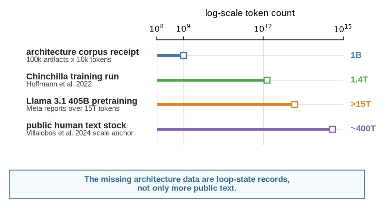
The token scale makes the contrast sharper. A broad corpus built from roughly fifty years of public computer-architecture, systems, and EDA literature might only be on the order of \(10^9\) tokens. A rough receipt is simple: \[ T_{\mathrm{arch\text{-}text}} \approx N_{\mathrm{artifacts}}\bar{t}_{\mathrm{artifact}} \approx 10^5 \times 10^4 \approx 10^9 \ \mathrm{tokens}. \] That sounds large, but it is small by web-scale pretraining standards. More importantly, it is incomplete in the wrong way. Papers preserve accepted claims far better than failed configurations, simulator flags, workload revisions, EDA reports, review arguments, and rejected alternatives. Architecture 2.0 therefore cannot treat “all architecture text” as the dataset. The dataset must include the loop state that made the text credible, and it must expose enough tacit judgment to make assumptions, exclusions, and rejection decisions inspectable.
Figure 4.1 puts that estimate on the same log-scale axis as three public AI-data anchors: Chinchilla’s 1.4-trillion-token training run, Meta’s report that Llama 3.1 405B was trained on more than 15 trillion tokens, and a public human-text-stock estimate on the order of hundreds of trillions of tokens (Hoffmann et al. 2022; Meta AI 2024; Villalobos et al. 2024). The point is not that architecture should race to scrape the web. The point is that even a generous public architecture-text estimate is tiny by modern pretraining standards, while the most important missing records are not ordinary text at all.
Hoffmann, Jordan, Sebastian Borgeaud, Arthur Mensch, et al. 2022. “Training Compute-Optimal Large Language Models.” Advances in Neural Information Processing Systems 35: 30016–30. https://doi.org/10.48550/arXiv.2203.15556.
Meta AI. 2024. Introducing Llama 3.1: Our Most Capable Models to Date. https://ai.meta.com/blog/meta-llama-3-1/.
Villalobos, Pablo, Anson Ho, Jaime Sevilla, Tamay Besiroglu, Lennart Heim, and Marius Hobbhahn. 2024. Will We Run Out of Data? Limits of LLM Scaling Based on Human-Generated Data. https://doi.org/10.48550/arXiv.2211.04325.
Table 4.1 makes the receipt explicit. It is not a measured corpus inventory. It is a scale check that separates the easy counts from the hard missing records. The multiplication that gives \(10^9\) tokens is deliberately simple; the point is that even a generous public-text corpus is small, and the public surfaces we can count most easily are not the same thing as architecture loop state.
| Receipt | Current value | What it supports | Caveat |
|---|---|---|---|
| Public architecture, systems, and EDA artifacts | \(10^5\) paper-equivalent artifacts | Order-of-magnitude basis for the \(10^9\)-token scale check. | Assumption for intuition; not a measured corpus boundary. |
| Tokens per paper-equivalent artifact | \(10^4\) tokens per artifact | Transparent multiplication: \(10^5 \times 10^4 = 10^9\). | Tokenization and artifact length vary; manuals and specifications can be much larger. |
| DBLP title pilot | 1,015 title records from selected ISCA, MICRO, HPCA, and ASPLOS years | Shows that public metadata is easy to collect and useful for trajectory signals. | Title-only pilot; not full text, artifacts, tool state, or design-loop evidence. |
| GitHub RTL language proxy | 141,288 Verilog repositories; 43,371 SystemVerilog repositories | Shows a large public RTL-adjacent surface that could seed artifact mining. | Broad language counts include small, toy, forked, stale, and non-architecture repositories. |
| GitHub RTL keyword proxy | 4,292 Verilog+“rtl” repositories; 1,657 SystemVerilog+“rtl” repositories | Gives a narrower proxy for RTL-oriented repositories. | Keyword-sensitive and unvalidated; it is still not a count of usable architecture design examples. |
| GitHub topic proxy | 353 computer-architecture-tagged Verilog repositories; 1,817 FPGA-tagged Verilog repositories | Shows that curated labels are much smaller than broad language counts. | Topic labels are voluntary, incomplete, and uneven across projects. |
| Missing loop-state records | Not counted | The highest-value architecture data are traces, configs, logs, reports, reviews, negative results, and rejected candidates. | Much of this state is private, tacit, uncodified, or discarded before publication. |
The useful lesson from the receipt is the mismatch. A title corpus can help map topic drift, but it cannot recover simulator flags, failed configurations, or review arguments. A Verilog repository count can show that public RTL-like material exists, but it does not say whether the repository contains a well-specified architecture decision, a reusable testbench, a valid workload, or evidence that rejected alternatives were considered. Architecture 2.0 therefore needs corpus building and representation design at the same time: more artifacts, but also better records of why those artifacts are credible.
The medical AI lineage is a useful comparison because it shows both the power and the limit of domain adaptation. BioBERT adapted a general language model to biomedical text; ClinicalBERT adapted representations to clinical notes; Med-BERT adapted BERT-style pretraining to structured electronic health records rather than ordinary prose (Lee et al. 2020; Huang et al. 2019; Rasmy et al. 2021). Those systems mattered because they treated the domain’s data format as a first-order problem. Chip design has its own instance. ChipNeMo adapts language models to hardware-design text with a custom tokenizer, domain-continued pretraining, and retrieval over internal corpora, then applies them to engineering question-answering, electronic-design-automation script drafting, and bug-report summarization (Liu et al. 2023). It demonstrates that domain adaptation pays off, and it illustrates the limit this chapter presses: it maps text to text, so it addresses the data-ingestion problem, not the closed design loop. Architecture must do the same domain work, but the representation burden is broader. A compute-subsystem design loop needs not only domain terms, but also executable tool state, workload provenance, constraints, multi-fidelity feedback, rejected alternatives, and decision authority. A paper corpus can bootstrap knowledge; it cannot by itself represent the design loop.
Lee, Jinhyuk, Wonjin Yoon, Sungdong Kim, et al. 2020. “BioBERT: A Pre-Trained Biomedical Language Representation Model for Biomedical Text Mining.” Bioinformatics 36 (4): 1234–40. https://doi.org/10.1093/bioinformatics/btz682.
Huang, Kexin, Jaan Altosaar, and Rajesh Ranganath. 2019. “ClinicalBERT: Modeling Clinical Notes and Predicting Hospital Readmission.” arXiv Preprint arXiv:1904.05342. https://arxiv.org/abs/1904.05342.
Rasmy, Laila, Yang Xiang, Ziqian Xie, Cui Tao, and Degui Zhi. 2021. “Med-BERT: Pretrained Contextualized Embeddings on Large-Scale Structured Electronic Health Records for Disease Prediction.” Npj Digital Medicine 4 (86). https://doi.org/10.1038/s41746-021-00455-y.
Liu, Mingjie, Teodor-Dumitru Ene, Robert Kirby, et al. 2023. ChipNeMo: Domain-Adapted LLMs for Chip Design. arXiv preprint arXiv:2311.00176. https://arxiv.org/abs/2311.00176.
Rajpurkar, Pranav, Jian Zhang, Konstantin Lopyrev, and Percy Liang. 2016. “SQuAD: 100,000+ Questions for Machine Comprehension of Text.” Proceedings of the 2016 Conference on Empirical Methods in Natural Language Processing, 2383–92. https://doi.org/10.18653/v1/D16-1264.
Wang, Alex, Amanpreet Singh, Julian Michael, Felix Hill, Omer Levy, and Samuel R. Bowman. 2018. “GLUE: A Multi-Task Benchmark and Analysis Platform for Natural Language Understanding.” Proceedings of the 2018 EMNLP Workshop BlackboxNLP: Analyzing and Interpreting Neural Networks for NLP, 353–55. https://doi.org/10.18653/v1/W18-5446.
Benchmark lineages such as SQuAD and GLUE teach a related lesson (Rajpurkar et al. 2016; Wang et al. 2018). They helped turn language understanding into repeatable evaluation objects: common inputs, common metrics, and comparable results. Architecture needs shared evaluation objects too, but an architecture “example” is rarely just a cheap labeled row. It may be a simulator run, a synthesis run, a physical-design report, a workload trace, a failed configuration, or an expert review tied to a specific fidelity level. The cost of a sample is therefore part of the representation problem, not an afterthought.
4.2 Sample Cost Is Architecture Data
In many benchmark settings, a sample is treated as an input-output pair: a question and answer, an image and label, a prompt and reference response. In an architecture design loop, a sample is better understood as a feedback event that changes what the loop believes. It might be a cycle-level simulation, a compiler report, a failed synthesis run, a power estimate, a rejected floorplan, an expert review, or a silicon measurement. Each event has a cost, fidelity, provenance, and commitment level.
Architecture sample. An architecture sample is any feedback event that changes the loop’s belief about a design candidate, including its cost, fidelity, provenance, assumptions, rejected-space coverage, and commitment level.
The vector does not collapse into one currency; its dimensions carry different units. It is a reminder that an architecture sample carries hidden state. A simulator point may require setup time, tool availability, license access, calibration work, human triage, and the opportunity cost of not evaluating another candidate. A post-layout result may carry higher fidelity but also higher latency and risk. A field deployment measurement may be authoritative for one population and irrelevant for another.
Concrete architecture tools span this range. Analytical mapping and dataflow models are designed for broad design-space exploration (Parashar et al. 2019; Kwon et al. 2019). Physical-design and verification flows expose the other end of the spectrum, where feedback can take hours or days and the human and engineering cost becomes part of the sample itself (Mirhoseini et al. 2021; Semiconductor Industry Association 2026; Bauer et al. 2020; Foster 2022). Table 4.2 is therefore not a tool taxonomy. It is a representation checklist: if the row changes, the loop must record different state.
Parashar, Angshuman, Priyanka Raina, Yakun Sophia Shao, et al. 2019. “Timeloop: A Systematic Approach to DNN Accelerator Evaluation.” 2019 IEEE International Symposium on Performance Analysis of Systems and Software, ISPASS, 304–15. https://doi.org/10.1109/ISPASS.2019.00042.
Kwon, Hyoukjun, Prasanth Chatarasi, Michael Pellauer, Angshuman Parashar, Vivek Sarkar, and Tushar Krishna. 2019. “Understanding Reuse, Performance, and Hardware Cost of DNN Dataflows: A Data-Centric Approach.” Proceedings of the 52nd Annual IEEE/ACM International Symposium on Microarchitecture, MICRO ’52, 754–68. https://doi.org/10.1145/3352460.3358252.
Semiconductor Industry Association. 2026. Chip Design and R&D. https://www.semiconductors.org/policies/chip-design/.
Bauer, Harald, Ondrej Burkacky, Peter Kenevan, Stephanie Lingemann, Klaus Pototzky, and Bill Wiseman. 2020. Semiconductor Design and Manufacturing: Achieving Leading-Edge Capabilities. McKinsey & Company report. https://www.mckinsey.com/industries/semiconductors/our-insights/semiconductor-design-and-manufacturing-achieving-leading-edge-capabilities.
Foster, Harry. 2022. Part 8: The 2022 Wilson Research Group Functional Verification Study. Verification Horizons, Siemens EDA. https://blogs.sw.siemens.com/verificationhorizons/2022/12/12/part-8-the-2022-wilson-research-group-functional-verification-study/.
| Feedback source | Latency / cost intuition | What it teaches | Record for reuse |
|---|---|---|---|
| Analytical model or mapper | Milliseconds to seconds; low direct cost; high model-risk exposure. | Useful for pruning and sensitivity checks, not final evidence. | Model assumptions, workload slice, constraints, and proxy-validity notes. |
| Trace, profile, or replay | Seconds to hours depending on capture and replay setup. | Workload provenance is part of the sample. | Trace version, sampling policy, software stack, and filtering choices. |
| Cycle-level simulation | Minutes to days depending on model detail and target workload. | Simulator evidence is scoped by abstraction, calibration, and unsupported states. | Simulator version, configuration, seeds, workload revision, and calibration notes. |
| RTL, gate, or EDA feedback | Hours to days when synthesis, timing, power, or physical feedback enters the loop. | High-fidelity samples are scarce and multiobjective. | Tool versions, constraints, process assumptions, waived warnings, and rejected candidates. |
| FPGA, emulation, or prototype | High setup and shared-resource cost; high throughput once mapped. | Speed changes observability and debugging semantics, not only wall-clock time. | Mapping constraints, observability limits, debug hooks, and queue/resource state. |
| Silicon or field telemetry | Weeks to years and high commitment. | Authoritative measurements still require context and human decision authority. | Population, deployment version, rollback policy, incident context, and decision owner. |
The timing side is multiplicative. A simulator is not slow in the abstract; it is slow relative to the target cycles the workload demands. For a target clock \(f_{\mathrm{target}}\), workload duration \(T_{\mathrm{workload}}\), and simulation throughput \(R_{\mathrm{sim}}\), the wall time is \[ T_{\mathrm{wall}} = \frac{N_{\mathrm{cycles}}}{R_{\mathrm{sim}}} = \frac{f_{\mathrm{target}}T_{\mathrm{workload}}}{R_{\mathrm{sim}}}. \] Table 4.3 gives the intuition for a 1 GHz target. The rates are illustrative, but the multiplication is the point: a loop can afford many cheap proxy samples, fewer cycle-level samples, and very few high-fidelity samples unless it has a disciplined plan for escalation and rejection.
| Target workload at 1 GHz | Target cycles | 1 kcycle/s | 100 kcycle/s | 10 MHz | 100 MHz |
|---|---|---|---|---|---|
| 1 ms | \(10^{6}\) | 16.7 min | 10 s | 0.1 s | 0.01 s |
| 1 s | \(10^{9}\) | 11.6 days | 2.8 h | 1.7 min | 10 s |
| 1 min | \(6\times 10^{10}\) | 1.9 years | 6.9 days | 1.7 h | 10 min |
| 1 h | \(3.6\times 10^{12}\) | 114 years | 1.1 years | 4.2 days | 10 h |
This cost structure changes how we should think about design spaces. A small co-design exercise with \(5 \times 4 \times 6 = 120\) candidates can sometimes be enumerated. A physical-design, compiler, mapping, or chiplet-integration space may be combinatorial, sequential, tool-bound, and partially invalid. Learning-assisted chip placement makes the point concrete: the design problem can be formulated as a learning problem, but the value of each sample depends on the representation of macros, nets, constraints, tool feedback, and placement validity (Mirhoseini et al. 2021); that result was later contested on its baselines and reproducibility (Chapter 7) (Cheng et al. 2023), which only sharpens the point. The architecture lesson is broader than placement. When samples are expensive, the dataset must record what each sample cost, what region of the space it informs, and what it rules out.
Mirhoseini, Azalia, Anna Goldie, Mustafa Yazgan, et al. 2021. “A Graph Placement Methodology for Fast Chip Design.” Nature 594 (7862): 207–12. https://doi.org/10.1038/s41586-021-03544-w.
Cheng, Chung-Kuan, Andrew B. Kahng, et al. 2023. “Assessment of Reinforcement Learning for Macro Placement.” Proceedings of the 2023 International Symposium on Physical Design (ISPD). https://doi.org/10.1145/3569052.3578926.
Chapter 6 returns to sample efficiency from the method side. The representation lesson comes first: if cost, fidelity, and rejected-space coverage are not recorded, a later optimizer cannot know whether it is learning the design space or merely collecting disconnected measurements.
4.3 Architecture Descriptions as Boundary Objects
An architecture description is a boundary object. It sits between human intent and tool action. It must be readable enough for architects to inspect, precise enough for tools to execute, and structured enough for agents or methods to modify without breaking the design contract.
At minimum, an architecture description should say what is being described, what hierarchy it assumes, what timing model or abstraction level is being used, what memory semantics matter, what workload scope is in bounds, what constraints must hold, and which tools can consume the description. For a memory hierarchy, this may include cache sizes, associativity, replacement policy, prefetching, coherence assumptions, bandwidth, latency, and workload mix. For an accelerator or compute subsystem, it may include supported operations, data layout, local storage, vector width, dataflow, quantization, compiler/runtime assumptions, and fallback behavior.
The important point is not that every representation must be one universal schema. Different loops need different representations. A paper-reading loop, a simulator-driven design-space exploration loop, an RTL-generation loop, and a post-silicon telemetry loop should not have identical records. But they do need explicit invariants. What fields must be present? Which fields can a method change? Which fields are read-only constraints? Which assumptions travel with a result? Which tool versions, seeds, and workload revisions are required for replay?
Without those boundaries, a representation becomes a prompt-shaped anecdote. It may sound plausible, but it cannot safely drive action.
4.4 Representation Debt and Structured Design Data
Architecture teams accumulate representation debt. The debt appears whenever important design state exists but is not captured in a durable, inspectable form. It may live in shell scripts, simulator flags, spreadsheet formulas, plotting notebooks, benchmark directories, issue threads, email, review slides, or the memory of the person who knows why one candidate was rejected. Some of the debt is tacit rather than textual: what an experienced architect chooses not to try, which proxy result they distrust, which corner case they ask about in review, and which risk they refuse to delegate.
This debt is manageable when a small team manually coordinates the loop. It becomes a technical failure when an AI system acts inside the loop. If a constraint is implicit, the method may violate it. If a simulator flag is hidden, the result may not be replayable. If rejected candidates are missing, the search may rediscover known failures. If workload provenance is unclear, the loop may optimize for the wrong distribution. If plots preserve only the winning candidate, the evidence trail cannot explain why alternatives were discarded.
TipField note: the result no one could rerun
A team reports a strong design-space result, then is asked to reproduce it six months later. The winning configuration survives in a plot, but the simulator version has moved, a default flag has changed, the workload trace has been re-cut, and the script that generated the run lived on a laptop that has since been reimaged. The number was real; the loop that produced it was not recorded. The fix is not heroics at reproduction time. It is recording the tool version, seed, flags, workload revision, and exact command as the run happens, so the result stays auditable after the people and machines move on.
Table 4.4 gives common sources of representation debt. The point is not to document everything for its own sake. The point is to capture enough state that a loop can compare, replay, reject, and revise.
| Artifact | What it enables | What it often hides | Failure mode |
|---|---|---|---|
| Paper or plot | Claim, result, and comparison. | Tool flags, failed candidates, tuning history. | Reproduce only the story, not the loop. |
| Workload trace | Concrete input behavior and measurements. | Coverage, versioning, sampling policy, privacy filters. | Optimize for an unrepresentative slice. |
| Simulator config | Replayable model setting. | Defaults, unsupported states, calibration limits. | Trust a number outside its valid scope. |
| RTL or EDA report | Implementation-facing feedback. | Process assumptions, constraints, waived warnings. | Accept an artifact that cannot close. |
| Review notes | Human judgment and rationale. | Tacit assumptions and discarded alternatives. | Lose why a decision was made. |
| Rejected candidate | Search boundary and negative evidence. | Why it failed and at what fidelity. | Rediscover known dead ends. |
4.5 QuArch as a Stress Test
QuArch is a useful stress test for this chapter because it starts from a real need: evaluating architecture knowledge in AI agents. A question-answering dataset can turn part of the literature into a structured evaluation object (Prakash et al. 2025b). The later QuArch reasoning benchmark makes the same point more explicit by organizing 2,671 expert-validated questions around recall, analysis, design, and implementation competencies (Prakash et al. 2025a). QuArch can ask whether a model recalls concepts, tracks architectural relationships, reasons over published claims, and avoids obvious domain mistakes. That is valuable. A field cannot build credible agents if the agents lack basic architectural knowledge.
Prakash, Shvetank et al. 2025b. “QuArch: A Question-Answering Dataset for AI Agents in Computer Architecture.” IEEE Computer Architecture Letters, ahead of print. https://doi.org/10.1109/LCA.2025.3541961.
Prakash, Shvetank et al. 2025a. QuArch: A Benchmark for Evaluating LLM Reasoning in Computer Architecture. https://arxiv.org/abs/2510.22087.
But QuArch also exposes the limit of paper-derived data. Papers preserve accepted claims better than they preserve design-loop state. They rarely contain every simulator configuration, rejected candidate, failed run, hidden constraint, calibration choice, or review argument. A model that answers questions over papers may know what a concept means and still lack the state needed to act inside a design loop. It may summarize a memory-system paper, but it does not necessarily know which candidates failed, which simulator flags were decisive, which workload slices were excluded, or which result would cause a human architect to reject the next proposal.
The lesson is not that question-answering datasets are insufficient and therefore unimportant. The lesson is that they occupy one layer. They help represent architectural knowledge. Architecture 2.0 also needs representations of experiments, tools, constraints, provenance, and negative traces. A reader should see QuArch as one example of bootstrapping the data layer, not as the whole data layer.
4.6 Toward Architecture World Models
Architecture world model. An architecture world model is the loop’s belief about how actions change architecture state and outcomes, including dynamics, costs, constraints, invalid-action rules, uncertainty, and decision policies.
This distinction matters. A simulator configuration is part of the representation. The simulator’s behavior, scope, calibration, and failure modes are part of the world model. A table of candidate parameters is representation. A surrogate that predicts latency or energy from those parameters is a world model. A set of design rules, expert heuristics, or physical constraints can also act as a world model.
Figure 4.2 gives the basic structure. A representation record contains workload traces, architecture descriptions, tool configurations, logs, constraints, and objectives. A world model contains state, action spaces, dynamics, costs, constraints, invalid-action rules, uncertainty, and decision policies. Tools return feedback; evidence updates both the representation and the world model.

There are several kinds of architecture world models. A simulator-backed world model uses a tool as the transition and feedback mechanism. A learned surrogate world model predicts outcomes from prior evaluations. A symbolic or constraint-based world model encodes invalid configurations, design rules, or physical limits. A hybrid world model combines these pieces: a simulator for selected candidates, a learned predictor for cheap screening, a rule system for invalid actions, and a human review policy for high-commitment decisions.
No world model is automatically credible. Each has a scope. Each has uncertainty. Each can be wrong under distribution shift, new workloads, different software stacks, tool changes, or higher-fidelity evaluation. The goal is not to pretend the world model is truth. The goal is to make its assumptions explicit enough that the loop can decide when to trust it, when to escalate fidelity, and when to reject its advice.
4.7 Provenance, Coverage, Labels, and Negative Traces
The most distinctive architecture data may be the data the field usually throws away. Published work tends to preserve accepted artifacts. Design loops also need rejected alternatives. A failed simulator run, invalid configuration, proxy win that fails at higher fidelity, abandoned floorplan, or unsupported-software path is not merely noise. It teaches the loop where the boundary lies.
Negative traces matter because architecture action spaces are full of invalid or misleading moves. A generated RTL fragment may be syntactically plausible but fail timing or violate an interface. A design-space search may find a candidate that looks good under a proxy but fails under a better power model. A benchmark result may improve because the workload slice is too narrow. A chiplet partition may appear modular but introduce unacceptable latency, thermal coupling, test complexity, or supply-chain risk.
Table 4.5 turns this point into a data schema. The purpose is to record what failed, what boundary it exposed, and how that evidence should change the next action in the loop.
| Negative trace | What it records | What the loop learns |
|---|---|---|
| Invalid configuration | Candidate violates constraints, tool schema, or interface contract. | Shrink or reshape the action space. |
| Proxy win that fails fidelity | Cheap metric improves, but stronger evaluation rejects it. | Calibrate proxies and require sensitivity checks. |
| Tool failure or crash | Simulator, synthesis, compiler, or harness cannot complete. | Separate design failure from environment failure. |
| Coverage gap | Workload, input, scenario, or architecture class was not represented. | Mark the evidence boundary before committing. |
| Rejected design rationale | Human review rejects a candidate for risk, maintainability, schedule, or integration. | Preserve architect judgment as training and audit data. |
Negative traces require provenance. A failed result without context is not very useful. The loop needs to know which workload, tool version, seed, parameters, constraints, and fidelity level produced the failure. It also needs coverage: what part of the design space, workload space, or evidence regime does this trace represent? Without provenance and coverage, negative traces become a pile of anecdotes. With them, they become architecture data.
4.8 When a Representation Becomes Actionable
A representation becomes actionable when it can safely support loop operations. It should define valid actions, expose relevant observations, carry constraints and objectives, record provenance, support replay, preserve uncertainty, separate feedback from evidence, and record what rejects a candidate. It should also say what remains a human decision.
This is a higher bar than asking whether a model can read it. A representation that can be summarized may still be useless for design. A representation that can be searched may still hide invalid actions. A representation that produces a score may still lack provenance. A representation that captures winning results but not rejected alternatives may teach the loop a biased view of the space.
For the lighthouse prompt, an actionable representation would not merely contain the prompt text. It would include the XRBench scenario, workload metadata, architecture parameters, software assumptions, power and process constraints, tool configurations, candidate set, feedback budget, evidence regime, negative traces, and rejection rules. Only then can the loop ask a bounded question: which candidate should be evaluated next, which evidence is strong enough, and which decision still belongs to the architect?
Chapter 5 takes the next step. Once state is represented, tools can become environments. They define what actions are legal, what feedback is returned, how expensive evaluation is, and what evidence a loop can produce.