8 Running the Loop: The Lighthouse Prompt, End to End
TipWhat this chapter gives you
After this chapter you can:
- instantiate and run a design-loop card on a concrete prompt, not merely fill it in;
- recognize proxy mismatch when the cheapest winner fails at higher fidelity;
- apply the commitment rule to stop at an honest evidence level;
- read the residue a loop leaves: evidence chain, negative traces, and the next evidence the decision needs.
The lecture has described what a credible loop must contain. It has not yet shown one turn. This chapter does that. It takes the lighthouse prompt, bounds it to a task small enough to run, and walks the loop through generation, prediction, escalation, rejection, and commitment. Every number here is illustrative and generated in code, not measured; the lesson is the shape of the loop, not the values.
Bounding the task comes first. “Design a low-power XR compute subsystem” is not a loop; it is a wish. The bounded task for this chapter is narrower: for one XRBench-class workload slice, choose among three compute organizations under a 3 W power envelope and an 8 ms per-frame real-time deadline, and return the surviving candidate with its evidence and its rejected alternatives. The candidates are a vector CPU extension, a tightly coupled accelerator, and a shared-memory SoC block. That is enough to make the loop turn.
8.1 Round One: Generate and Screen on a Proxy
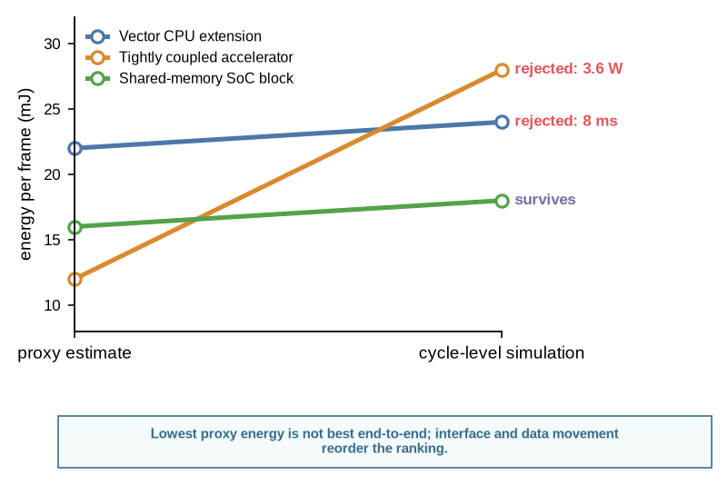
The loop begins cheaply. A generator proposes the three organizations, and an analytic proxy, a pre-RTL estimator in the spirit of Aladdin or a dataflow model like Timeloop (Shao et al. 2014; Parashar et al. 2019), estimates latency and energy per frame in milliseconds and millijoules. The proxy is fast and ignores most data movement, so it flatters designs that keep arithmetic local. At this fidelity the tightly coupled accelerator looks best: it posts the lowest energy and latency because the proxy never charges it for moving data in and out.
Shao, Yakun Sophia, Brandon Reagen, Gu-Yeon Wei, and David Brooks. 2014. “Aladdin: A Pre-RTL, Power-Performance Accelerator Simulator for Rapid Design Space Exploration.” Proceedings of the 41st Annual International Symposium on Computer Architecture (ISCA). https://doi.org/10.1109/ISCA.2014.6853196.
Parashar, Angshuman, Priyanka Raina, Yakun Sophia Shao, et al. 2019. “Timeloop: A Systematic Approach to DNN Accelerator Evaluation.” 2019 IEEE International Symposium on Performance Analysis of Systems and Software, ISPASS, 304–15. https://doi.org/10.1109/ISPASS.2019.00042.
A proxy result is feedback, not evidence. It is enough to keep all three candidates alive and to rank them for the next, more expensive stage. It is not enough to choose. The loop records the proxy ranking and escalates.
8.2 Round Two: Escalate to Simulation
Cycle-level simulation, a gem5-class model (Binkert et al. 2011), is the first stage that models memory traffic. It is slower and scarcer than the proxy, so the loop spends it only on the candidates that survived screening. The result is the central lesson of the chapter:
Binkert, Nathan, Bradford Beckmann, Gabriel Black, et al. 2011. “The Gem5 Simulator.” ACM SIGARCH Computer Architecture News 39 (2): 1–7. https://doi.org/10.1145/2024716.2024718.
Table 8.1 runs the comparison.
| Candidate | Proxy lat / energy | Sim lat / energy | Power | Verdict |
|---|---|---|---|---|
| Vector CPU extension | 9.0 ms / 22 mJ | 9.5 ms / 24 mJ | 2.1 W | rejected: misses 8 ms deadline |
| Tightly coupled accelerator | 4.5 ms / 12 mJ | 8.8 ms / 28 mJ | 3.6 W | rejected: over 3 W envelope |
| Shared-memory SoC block | 6.0 ms / 16 mJ | 6.5 ms / 18 mJ | 2.8 W | survives to RTL study |
The accelerator that won on the proxy collapses under simulation. Once data movement is charged, its energy rises above every alternative and its latency loses most of its lead. This is proxy mismatch made concrete: the loop was optimizing the measurement it could see, not the objective it cared about. The failed candidate is not deleted. It is recorded as a negative trace, with the fidelity level at which the proxy win disappeared, so a later loop does not rediscover it. Figure 8.1 shows the reorder.
8.3 Round Three: Reject on the Envelope
Simulation also exposes a harder gate. The tightly coupled accelerator does not merely lose on energy; its power model puts it over the 3 W envelope. That is a constraint, not a metric, so no amount of latency advantage rescues it. The rejection is the commitment rule from the trust chapter doing its work: a candidate advances only if it is valid, its evidence clears the threshold for the stage, and its residual risk is acceptable.
The accelerator’s failure has a familiar shape. Its attraction was a large local speedup, but the interface and data-movement cost to reach it dominated the end-to-end result. The next chapter makes this precise with an accelerator performance model; the loop-level lesson is simpler: price the interface before believing the local win.
8.4 Round Four: Commit at an Honest Level
One candidate survives the deadline and the envelope. It is tempting to call that a result. It is not, yet. The evidence behind it is a cycle-level simulation and a power model, which support an experimental commitment, not an implementation or a tapeout. The architect’s decision is therefore bounded: advance the surviving organization to an RTL study where synthesis, timing, and a stronger power estimate can confirm or reject it, and hold the other two as recorded negative traces.
This is the difference between an answer and a defensible answer. The loop did not produce a chip. It produced a surviving candidate, the evidence that supports it, the alternatives that failed and why, and the next evidence the decision needs. That is what the lighthouse prompt was always asking for: a design-space report with evidence and rejected alternatives, not a one-shot generation.
8.5 What the Loop Leaves Behind
The residue of one turn is the reusable artifact. The loop leaves a filled design-loop card, an evidence chain that records the fidelity at each stage, two negative traces with the reasons they failed, and an explicit open question for the next stage. Another architect can read that residue and reconstruct why the surviving candidate advanced, why the others did not, and what would overturn the decision.
That is the test the rest of the lecture has been building toward. The reader should now be able to take a new project and do three things: name the loop, judge whether its evidence matches its commitment level, and state what remains a human decision. The next chapter generalizes this single worked loop into the patterns that recur across the stack, from fast software loops to high-commitment silicon-facing work.
ImportantArchitect’s checkpoint
Running your own loop, ask:
- Is the task bounded enough that a candidate can actually be rejected?
- When a cheap proxy and a stronger check disagree, which do I trust, and why?
- At what commitment level does my evidence actually let me stop?