6 Methods for Generation, Prediction, and Optimization
TipWhat this chapter gives you
After this chapter you can:
- match a method role (generate, predict, optimize, critique, verify) to an architecture task;
- state a method claim as object, action, feedback, and rejection condition;
- assess hardware awareness as a staged capability, not the use of hardware vocabulary;
- choose a method by loop conditions rather than by fashion.
Chapter 5 defined the environment: the place where actions are taken and feedback is observed. This chapter asks which methods belong inside that environment. The answer is not a ranking of current models or agent frameworks. It is a discipline for matching method roles to architecture work.
The distinction matters. A model that can generate plausible schedules, configuration files, code fragments, RTL snippets, or design prose may be useful for drafting alternatives, but weak for choosing among them. A surrogate may predict latency or energy well inside a calibrated accelerator design region, but fail outside the sampled space. Bayesian optimization may spend scarce simulator or synthesis evaluations carefully, but only if the action space and objective are well formed. Reinforcement learning may be attractive for placement, scheduling, or adaptive control, but dangerous when invalid actions are common and feedback is delayed. A critic may be more valuable than a generator when the urgent problem is exposing missing workload evidence, not proposing more candidates.
Architecture 2.0 therefore treats methods as roles in a compound design system. A credible loop might include a generator that proposes candidates, a predictor that estimates behavior, an optimizer that selects the next experiment, a critic that challenges assumptions, a verifier that checks constraints, and a human architect who decides whether the evidence is strong enough to proceed. The method question is not “Which AI system is best?” It is “Which role is needed, what feedback can support it, and what evidence would make its output credible?”
Machine learning for architecture did not begin with recent agents. A useful historical shorthand is prediction, optimization, and generation. Prediction appears in regression models, learned surrogates, and calibrated performance or power estimators. Optimization appears in Bayesian optimization, autotuning, reinforcement learning, and search over compiler, mapping, placement, or architecture parameters. Generation now appears in natural-language-to-code, RTL, test, configuration, and design-report workflows. The shorthand is useful because it gives proper credit to earlier work. It is also incomplete. The Architecture 2.0 question is how these roles compose with critique, repair, verification, provenance, negative traces, and human rejection authority inside one explicit loop.
6.1 Match the Method to the Architecture Task
The first step is to name the architecture task. Design-space exploration, workload characterization, benchmark construction, code generation, RTL repair, compiler/runtime tuning, accelerator search, chiplet partitioning, physical-design assistance, and evidence critique are not the same problem. They expose different state, allow different actions, tolerate different errors, and require different feedback.
This is why environment work such as ArchGym is important: it makes method comparisons meaningful by defining tasks, actions, observations, workloads, and feedback (Krishnan et al. 2023). But even a shared environment does not decide which method role is appropriate. The role depends on what the loop is trying to accomplish.
Krishnan, Srivatsan et al. 2023. “ArchGym: An Open-Source Gymnasium for Machine Learning Assisted Architecture Design.” Proceedings of the 50th Annual International Symposium on Computer Architecture, ISCA ’23. https://doi.org/10.1145/3579371.3589049.
Figure 6.1 shows the chapter’s working map. The same architecture loop can contain several method roles, but each role has a different claim and a different evidence requirement.

Table 6.1 gives the checklist form. The table is deliberately phrased as questions because method choice should be defended in architecture terms, not only in machine-learning terms.
| Role | Architecture use | Evidence needed | Failure mode |
|---|---|---|---|
| Generate | Propose configs, specs, code, RTL fragments, test benches, design reviews, or hypotheses. | Validity checks, constraints, provenance, and human review. | Plausible but invalid candidates. |
| Predict | Estimate performance, energy, area, latency, reliability, or cost before full evaluation. | Calibration, uncertainty, coverage, and held-out checks. | Confident extrapolation outside support. |
| Optimize | Choose the next candidate or region of the space to evaluate. | Objective, constraints, feedback budget, and stopping rule. | Gaming the proxy or missing the real tradeoff. |
| Critique/repair | Find weak assumptions, missing evidence, invalid actions, or broken artifacts. | Access to artifacts, claims, evidence, and rejection rules. | Polished explanations without authority to reject. |
| Verify | Check constraints, invariants, tests, tool outputs, and evidence chains. | Independent checks, provenance, and escalation rules. | Treating one tool pass as final truth. |
The discipline behind the table is simple: a method claim is incomplete until it names the architecture object being changed or estimated, the interface through which the action is legal, the feedback that supports the claim, and the condition that can reject it.
Object-action-evidence rule. State every method claim as: this role acts on this architecture object through this interface, receives this feedback, and can be rejected by this evidence.
Table 6.2 gives concrete examples. The same method family can be reasonable or unreasonable depending on which object it touches and what can say no. A generator that proposes benchmark questions is different from one that proposes RTL. A predictor that ranks early simulator configurations is different from one that claims final power. An optimizer that chooses the next cheap proxy run is different from one that commits a physical-design change.
| Role | Object to name | Feedback to require | Rejection condition |
|---|---|---|---|
| Generate | Workload variant, simulator config, tensor schedule, kernel, RTL fragment, EDA constraint, or design-loop card. | Parser, compiler, simulator, test harness, constraint checker, or human review. | Invalid syntax, unsupported action, wrong output, violated constraint, or missing provenance. |
| Predict | Latency, energy, area, memory traffic, timing risk, thermal behavior, queueing delay, or deployment impact. | Calibration data, uncertainty, coverage region, held-out checks, and fidelity label. | Out-of-support query, counterexample, proxy mismatch, or uncalibrated extrapolation. |
| Optimize | Next design point, parameter region, schedule, dataflow, mapping, placement move, or experiment allocation. | Objective, constraints, feedback budget, cost model, and stopping rule. | Proxy gaming, infeasible candidate, lost Pareto tradeoff, or exhausted evidence budget. |
| Critique/repair | Benchmark claim, simulator log, configuration file, test bench, source packet, evidence table, or rejected alternative. | Access to artifact provenance, claims, assumptions, and comparison baseline. | Missing workload coverage, stale tool version, unsupported conclusion, or unresolved failure. |
| Verify/explain | Invariant, interface contract, numerical tolerance, synthesis constraint, regression result, or evidence chain. | Independent checks, replayable commands, tool logs, and escalation record. | Failed check, inconsistent evidence, weak fidelity, or architect refusal to commit. |
6.2 Hardware Awareness as Staged Capability
Hardware awareness is not the same as using hardware vocabulary. A generated proposal can mention caches, vector units, power targets, or a process node and still be unaware of the architectural consequences of those terms.
Hardware awareness. In this lecture, hardware awareness means that a method or agent can represent hardware-relevant constraints, act within a valid hardware/software design space, obtain feedback from appropriate tools or measurements, and expose evidence that can reject its own output.
This definition matters because Architecture 2.0 methods will often generate or revise artifacts near the hardware/software boundary: kernels, compiler settings, accelerator configurations, RTL fragments, memory-system choices, placement constraints, or design reports. Hardware-aware neural architecture search already shows the value of putting latency, energy, memory footprint, and target-device cost into the search problem (Benmeziane et al. 2021). Architecture 2.0 uses a broader version of the same discipline: the question is not whether an artifact sounds hardware-aware, but what level of hardware-aware action and evidence the loop can support.
Benmeziane, Hadjer, Kaoutar El Maghraoui, Hamza Ouarnoughi, Smail Niar, Martin Wistuba, and Naigang Wang. 2021. “Hardware-Aware Neural Architecture Search: Survey and Taxonomy.” Proceedings of the Thirtieth International Joint Conference on Artificial Intelligence, 4322–29. https://doi.org/10.24963/ijcai.2021/592.
Figure 6.2 gives the working capability map. The levels are cumulative as an assessment vocabulary, but they are not a claim that every system improves along one monotone axis. A tool wrapper may compile and profile without having a strong performance model. A calibrated surrogate may estimate uncertainty without directly controlling a tool. The staging is useful because it forces the reader to ask which capability a method actually has, which capability it lacks, and what the loop is allowed to do with the result.
Vocabulary awareness is useful, but it only names the objects. Constraint awareness applies declared budgets and limits such as power, area, latency, memory, precision, reliability, and process assumptions. Performance-model awareness reasons about the mechanisms that drive cost: data movement, locality, bandwidth, occupancy, parallelism, pipelines, and communication. Tool and environment awareness connects those mechanisms to compilers, profilers, simulators, synthesis reports, and failed runs. Evidence awareness adds calibration, uncertainty, proxy mismatch, fidelity, and negative traces. Commitment-boundary awareness is the highest level because the method can state what it is allowed to decide, what must be escalated, and why.
Functional correctness is cross-cutting, not optional. Once a loop changes an executable or synthesizable artifact, tests, reference outputs, formal checks, type or interface checks, synthesis constraints, numerical tolerances, or expert review must be able to reject it before performance claims matter.

Table 6.3 makes the assessment explicit. Each level should be judged by what the method may change, what feedback supports that change, and what can reject it.
| Capability | What it may change | Feedback needed | Rejection authority |
|---|---|---|---|
| Vocabulary | Terms in prompts, reports, or design notes. | Human review of meaning and misuse. | Architect rejects fluent but empty claims. |
| Constraint | Candidate fields within declared budgets or limits. | Bounds, static checks, invalid-action filters, and feasibility rules. | Constraint violation or illegal action. |
| Performance model | Rankings, estimates, or parameter choices inside model support. | Calibration, sensitivity, residuals, and held-out checks. | Model miss, counterexample, or out-of-support query. |
| Tool/environment | Code, configs, kernels, traces, or tool-invoked candidates. | Compile, run, profile, simulate, synthesize, and log tool outcomes. | Failed test, tool error, profile regression, or invalid artifact. |
| Evidence and calibration | Confidence, evidence strength, and escalation recommendations. | Multi-fidelity comparison, uncertainty, provenance, and negative traces. | Proxy mismatch, weak provenance, or fidelity failure. |
| Commitment boundary | Accept, revise, reject, or escalate recommendation. | Evidence ledger, rollback cost, risk, and review context. | Human architect or independent verification refuses commitment. |
A kernel-generation loop that can compile, test, and profile generated kernels has tool awareness. It does not automatically have evidence awareness unless the loop records numerical correctness, speedup distributions, portability, rejected candidates, and proxy mismatch. A design-space agent that can propose accelerator parameters has constraint awareness only if invalid actions are blocked or rejected. It has commitment-boundary awareness only if it can connect workload intent, hardware resource limits, compiler/runtime assumptions, fidelity gates, and human decision points into one accountable loop. Here, “performance model” means a cheap analytical, learned, or surrogate estimator used before live tool execution. A simulator such as gem5 can itself be a tool environment when the loop invokes it, records configurations and outputs, and treats its result as feedback rather than as an abstract ranking.
6.3 Generation: Proposing Candidates and Artifacts
Generation is the most visible role because it is easy to demonstrate. A method can draft an architecture description, propose a simulator configuration, generate code, produce a test bench, write a design-review summary, suggest a memory hierarchy, sketch an accelerator interface, or enumerate hypotheses about a workload. In the lighthouse example, generation might propose a set of candidate vector widths, local memory sizes, data layouts, or CPU/accelerator partitions for the XRBench workload.
The danger is to mistake candidate generation for design. Generated artifacts are useful when they expand the set of possibilities, expose alternatives, or accelerate tedious translation. They are not credible merely because they are well formed. The loop still needs validity checks, tool execution, evidence, rejected alternatives, and human decision.
This distinction keeps Architecture 2.0 from becoming prompt-to-chip rhetoric. A generated RTL fragment is not an architecture result. A generated parameter set is not a design-space conclusion. A generated benchmark question is not a validated workload. Generation earns its place when it feeds a loop that can test, reject, compare, and revise.
WarningFallacy: generation is design
It is tempting to treat a fluent generated artifact, an RTL fragment, a config, a benchmark question, as a result. It is not. A generated artifact is a proposal; it becomes a result only after the loop tests it, prices its evidence, compares it against a baseline, and an architect accepts the commitment. Generation that is not embedded in a loop that can reject it is demonstration, not design.
The strongest near-term use of generation may be breadth. It can propose candidate decompositions, list assumptions, create alternative experiment plans, translate design intent into structured records, or draft the first version of a design-loop card. Those outputs are valuable because they give the architect more structured material to inspect. They become dangerous only when the loop treats them as decisions.
Kernel generation is a useful concrete case because it isolates the software and code-generation facet of the lighthouse prompt. The XRBench subsystem only matters if kernels, libraries, runtime paths, and target-specific code can be generated, checked, and maintained. KernelBench asks whether language models can generate correct and efficient GPU kernels for PyTorch workloads (Ouyang et al. 2025). The Architecture 2.0 lesson is not that kernel generation solves hardware/software co-design. It is that generation becomes meaningful only when it is embedded in a harness that can compile, run, test, profile, compare against a baseline, reject wrong outputs, and preserve negative traces. Follow-on kernel-generation benchmarks make the lesson sharper: multi-platform settings expose backend and portability contracts (Wen et al. 2025), while category-aware analyses show that correctness, task structure, numerical contracts, and efficiency can diverge (Wang et al. 2026). That is precisely why generation is a role in a loop, not the loop itself.
Ouyang, Anne, Simon Guo, Simran Arora, et al. 2025. “KernelBench: Can LLMs Write Efficient GPU Kernels?” arXiv Preprint arXiv:2502.10517, ahead of print. https://doi.org/10.48550/arXiv.2502.10517.
Wen, Zhongzhen, Yinghui Zhang, Zhong Li, Zhongxin Liu, Linna Xie, and Tian Zhang. 2025. “MultiKernelBench: A Multi-Platform Benchmark for Kernel Generation.” arXiv Preprint arXiv:2507.17773, ahead of print. https://doi.org/10.48550/arXiv.2507.17773.
Wang, Han, Jintao Zhang, Kai Jiang, Haoxu Wang, Jianfei Chen, and Jun Zhu. 2026. “KernelBenchX: A Comprehensive Benchmark for Evaluating LLM-Generated GPU Kernels.” arXiv Preprint arXiv:2605.04956, ahead of print. https://doi.org/10.48550/arXiv.2605.04956.
Blocklove, Jason, Siddharth Garg, Ramesh Karri, and Hammond Pearce. 2023. “Chip-Chat: Challenges and Opportunities in Conversational Hardware Design.” 2023 ACM/IEEE 5th Workshop on Machine Learning for CAD (MLCAD), 1–6. https://doi.org/10.1109/MLCAD58807.2023.10299874.
The same discipline appears closer to hardware. Chip-Chat reports a conversational loop in which a language model drafts Verilog, open-source simulation and synthesis tools check it, the resulting errors are fed back for revision, and a small processor design is carried as far as fabrication (Blocklove et al. 2023). The interesting part is not that a model produced Verilog. It is that the loop became trustworthy only because a parser, a simulator, and a synthesis flow could each reject a draft, and a human stayed in the conversation to decide when a candidate was good enough to commit. Generation supplied breadth; the environment and the architect supplied the authority to reject.
6.4 Prediction: Estimating Behavior before Full Evaluation
Prediction is central because architecture feedback is expensive. Long before recent foundation models, architects used statistical and machine-learning models to reduce the cost of exploring large design spaces. Regression models for microarchitectural performance and power, and predictive modeling for large architectural design spaces, are part of this lineage (Lee and Brooks 2006; Ipek et al. 2006).
Lee, Benjamin C., and David M. Brooks. 2006. “Accurate and Efficient Regression Modeling for Microarchitectural Performance and Power Prediction.” Proceedings of the 12th International Conference on Architectural Support for Programming Languages and Operating Systems, ASPLOS XII, 185–94.
Ipek, Engin, Sally A. McKee, Bronis R. de Supinski, Martin Schulz, and Rich Caruana. 2006. “Efficiently Exploring Architectural Design Spaces via Predictive Modeling.” Proceedings of the 12th International Conference on Architectural Support for Programming Languages and Operating Systems, ASPLOS XII, 195–206. https://doi.org/10.1145/1168857.1168882.
The prediction role is not limited to performance. A predictor might estimate energy, area, latency, reliability, queueing behavior, memory traffic, thermal behavior, compile time, implementation feasibility, or deployment impact. It might be a regression model, a learned surrogate, a calibrated analytic model, a simulator-backed approximation, or a hybrid that combines domain structure with data.
The key requirement is uncertainty. A point estimate is useful only if the loop understands where it is valid. Has the predictor seen similar workload regions? Does it extrapolate across a new memory behavior, vector width, or technology assumption? Does it report confidence? Is it calibrated against a higher-fidelity source? Does it preserve enough provenance to explain why a candidate was trusted?
There is a rigorous way to make this concrete. Conformal prediction turns any surrogate, regardless of its internals, into one that emits calibrated prediction sets: intervals that contain the true value with a user-chosen probability under only an exchangeability assumption (Angelopoulos and Bates 2021). For an architecture loop this converts “report confidence” from a slogan into an operation. The predictor returns not a point latency or energy but an interval, and the loop escalates to higher fidelity whenever that interval straddles a constraint, such as the 3 W envelope, or grows wider than the decision can tolerate. The guarantee is distribution-free, so it survives the non-Gaussian residuals architecture surrogates actually produce, and it degrades visibly under distribution shift, which is exactly when a proxy should not be trusted.
Angelopoulos, Anastasios N., and Stephen Bates. 2021. A Gentle Introduction to Conformal Prediction and Distribution-Free Uncertainty Quantification. arXiv preprint arXiv:2107.07511. https://arxiv.org/abs/2107.07511.
For the lighthouse prompt, a predictor could help screen candidate compute subsystems before full simulation or synthesis. But the evidence burden depends on the decision. A rough predictor may be enough to discard obviously bad candidates. It is not enough to claim that a design meets a 3 W target on a 3 nm-class low-power mobile process. The stronger the commitment, the stronger the calibration and fidelity requirement.
6.5 Optimization: Learning the Design Space
Optimization is often framed as search: find the best point under an objective. Architecture needs a richer formulation. The useful goal is to learn the design space well enough to make a defensible decision under limited feedback. That may mean finding a Pareto region, identifying a constraint boundary, understanding a sensitivity, ruling out a class of candidates, or deciding which expensive experiment is worth running next.
Bayesian optimization is attractive for Architecture 2.0 because it was built for expensive black-box functions and sequential experimentation (Jones et al. 1998; Snoek et al. 2012). It encourages the loop to trade off exploration and exploitation, to reason about uncertainty, and to spend evaluations where they are likely to matter. Those properties align naturally with architecture settings where simulator, synthesis, or measurement runs are costly.
Jones, Donald R., Matthias Schonlau, and William J. Welch. 1998. “Efficient Global Optimization of Expensive Black-Box Functions.” Journal of Global Optimization 13 (4): 455–92. https://doi.org/10.1023/A:1008306431147.
Snoek, Jasper, Hugo Larochelle, and Ryan P. Adams. 2012. “Practical Bayesian Optimization of Machine Learning Algorithms.” Advances in Neural Information Processing Systems 25: 2951–59.
Mirhoseini, Azalia, Anna Goldie, Mustafa Yazgan, et al. 2021. “A Graph Placement Methodology for Fast Chip Design.” Nature 594 (7862): 207–12. https://doi.org/10.1038/s41586-021-03544-w.
Cheng, Chung-Kuan, Andrew B. Kahng, et al. 2023. “Assessment of Reinforcement Learning for Macro Placement.” Proceedings of the 2023 International Symposium on Physical Design (ISPD). https://doi.org/10.1145/3569052.3578926.
Reinforcement learning is attractive when the problem is sequential: placement decisions, scheduling policies, adaptive control, or multi-stage design flows. The chip-floorplanning literature gives a prominent, and contested, example of posing a chip design subproblem as a learning problem (Mirhoseini et al. 2021); independent baselines later challenged the result (Chapter 7) (Cheng et al. 2023). The important lesson for this lecture is not that every architecture task should become RL. It is that method choice depends on state, action, transition, feedback, and commitment structure.
A less contested example narrows the design space until the environment can supply real rejection authority. PrefixRL casts the design of parallel-prefix arithmetic circuits, such as adders, as a reinforcement-learning problem with logic synthesis in the loop, so every proposed circuit is scored by an actual synthesis run rather than a hand-built proxy (Roy et al. 2021). The reported circuits reached the area-delay Pareto frontier of a production design flow, and the resulting arithmetic units were adopted in shipping GPU silicon. The contrast with the placement dispute is the lesson, not the leaderboard: the same method family is contested when its reward is a fast proxy and defensible when a bounded action space lets a high-fidelity instrument reject every candidate. Method choice is inseparable from what the environment can verify.
Roy, Rajarshi, Jonathan Raiman, Neel Kant, et al. 2021. “PrefixRL: Optimization of Parallel Prefix Circuits Using Deep Reinforcement Learning.” Proceedings of the 58th ACM/IEEE Design Automation Conference (DAC), DAC ’21, 853–58. https://doi.org/10.1109/DAC18074.2021.9586094.
Ansel, Jason, Shoaib Kamil, Kalyan Veeramachaneni, et al. 2014. “OpenTuner: An Extensible Framework for Program Autotuning.” Proceedings of the 23rd International Conference on Parallel Architectures and Compilation (PACT), 303–15. https://doi.org/10.1145/2628071.2628092.
Zheng, Lianmin et al. 2020. “Ansor: Generating High-Performance Tensor Programs for Deep Learning.” 14th USENIX Symposium on Operating Systems Design and Implementation, 863–79.
Autotuning and compiler optimization provide another useful precedent. General program-autotuning frameworks such as OpenTuner (Ansel et al. 2014), and tensor-program optimizers such as AutoTVM and Ansor, share a loop structure worth naming: a learned cost model proposes promising candidates, the loop compiles and measures the strongest of them on real hardware, and those measurements correct the cost model for the next round (Chen et al. 2018; Zheng et al. 2020). That is an active-learning loop running in production: the cheap proxy is never trusted alone, because high-fidelity feedback continually re-grounds it. These systems are not identical to microarchitecture design, but they are lighthouse facets rather than unrelated detours. Floorplanning stresses high-commitment physical feedback; autotuning stresses the compiler/runtime path that makes specialization usable. Both illustrate a durable pattern: a method is powerful when it is embedded in an environment that exposes legal actions, measures feedback, updates a cost model, and records results.
The optimizer should therefore be evaluated by what it learns and what it can explain, not only by its best score. Did it discover a robust region? Did it identify a proxy mismatch? Did it spend high-fidelity evaluations carefully? Did it preserve rejected alternatives? Did it show why one candidate was chosen over another? If the answer is no, the loop may have optimized a number without improving architectural understanding.
6.6 Sample Efficiency under Expensive Feedback
Sample efficiency is one of the reasons architecture is a hard AI domain. Many AI settings assume abundant feedback. Architecture often has the opposite shape: a small number of high-fidelity runs, a larger number of medium-fidelity simulations, many cheap proxies, and a long tail of hidden costs such as expert review, tool setup, debugging, and license availability.
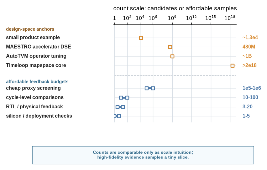
Figure 6.3 turns that mismatch into a count-scale picture. The upper rows reuse the design-space anchors from Chapter 2: the small product example from this book, the MAESTRO accelerator DSE scale, AutoTVM-style operator tuning spaces, and the core Timeloop mapspace expression (Kwon et al. 2019; Chen et al. 2018; Parashar et al. 2019). The lower rows reuse the representative feedback budgets from Chapter 5. These counts are not identical scientific quantities. The point is the scale mismatch: high-fidelity architecture evidence can touch only a tiny slice of the plausible candidate space, so methods must decide what can be screened by proxies, what should be escalated, and what rejected regions must be recorded.
Kwon, Hyoukjun, Prasanth Chatarasi, Michael Pellauer, Angshuman Parashar, Vivek Sarkar, and Tushar Krishna. 2019. “Understanding Reuse, Performance, and Hardware Cost of DNN Dataflows: A Data-Centric Approach.” Proceedings of the 52nd Annual IEEE/ACM International Symposium on Microarchitecture, MICRO ’52, 754–68. https://doi.org/10.1145/3352460.3358252.
Chen, Tianqi, Lianmin Zheng, Eddie Yan, et al. 2018. “Learning to Optimize Tensor Programs.” Advances in Neural Information Processing Systems 31.
Parashar, Angshuman, Priyanka Raina, Yakun Sophia Shao, et al. 2019. “Timeloop: A Systematic Approach to DNN Accelerator Evaluation.” 2019 IEEE International Symposium on Performance Analysis of Systems and Software, ISPASS, 304–15. https://doi.org/10.1109/ISPASS.2019.00042.
Chapter 4 treated sample cost as data the representation must carry. Here the same idea becomes a method-selection criterion. A sample is any feedback event that changes what the loop believes: a simulator result, tool warning, failed run, synthesis report, benchmark measurement, expert rejection, or higher-fidelity validation. The loop should not maximize sample count. It should maximize decision value per unit cost: \[ V_{\mathrm{sample}} \approx \frac{\Delta D}{C_{\mathrm{sample}}}, \] where \(\Delta D\) denotes the change in decision confidence, rejected-space coverage, or evidence strength produced by that sample. Neither term is directly measurable; the relation is a way to rank candidate experiments by what they would resolve, not a quantity the loop should try to maximize.
This heuristic has a rigorous counterpart. Bayesian optimization makes the choice of the next sample an explicit acquisition function over a surrogate’s posterior, and GP-UCB gives that choice a no-regret guarantee under stated assumptions, so the loop can defend why it sampled where it did rather than appealing to intuition (Srinivas et al. 2010). Multi-fidelity Bayesian optimization goes one step further and treats the fidelity level itself as a decision variable: it chooses not only which candidate to evaluate but whether to spend a cheap proxy or an expensive simulation on it, exactly the choice the fidelity ladder poses (Kandasamy et al. 2017). The architecture loop rarely needs the full apparatus, but naming it matters: sample efficiency is a solved problem in form, and a loop that ignores it is leaving evidence on the table.
Srinivas, Niranjan, Andreas Krause, Sham M. Kakade, and Matthias Seeger. 2010. “Gaussian Process Optimization in the Bandit Setting: No Regret and Experimental Design.” Proceedings of the 27th International Conference on Machine Learning (ICML), 1015–22. https://arxiv.org/abs/0912.3995.
Kandasamy, Kirthevasan, Gautam Dasarathy, Jeff Schneider, and Barnabás Póczos. 2017. “Multi-Fidelity Bayesian Optimisation with Continuous Approximations.” Proceedings of the 34th International Conference on Machine Learning (ICML), PMLR, vol. 70: 1799–808. https://proceedings.mlr.press/v70/kandasamy17a.html.
Table 6.4 gives a simple way to think about the regimes. The numbers are illustrative, not prescriptions. The point is that method choice changes when feedback is measured in milliseconds, minutes, hours, weeks, or silicon cycles.
| Regime | Typical setting | Method implication | Evidence discipline |
|---|---|---|---|
| Many cheap proxy runs | Analytic models, rough estimators, compiler hints. | Broad search, candidate generation, surrogate pretraining. | Track proxy validity and avoid overfitting the cheap metric. |
| Hundreds of simulations | Simulator-backed DSE or workload sweeps. | Bayesian optimization, active learning, transfer, sensitivity analysis. | Record seeds, configs, workloads, and failed runs. |
| Tens of expensive tool runs | Synthesis, physical design, emulation, or hardware-in-the-loop. | Strong priors, staged gates, human filtering, small candidate sets. | Require calibration and explicit rejection rules. |
| Few high-commitment checks | Silicon, deployment, fleet experiments, or customer workloads. | Critique, evidence organization, conservative recommendations. | Human decision and audit trail dominate. |
This is where negative traces matter. Failed simulations, invalid candidates, timeouts, rejected configurations, and proxy mismatches are not noise to be discarded. They are information about the boundary of the design space. A sample-efficient loop should learn from what failed, not only from the points that produced clean plots.
Sample efficiency also depends on representation. If the environment logs only final scores, the method cannot reuse much. If it records workload metadata, candidate structure, tool warnings, failure reasons, and fidelity level, then each sample teaches more. Chapter 4 and Chapter 5 are therefore not preliminaries to methods. They determine whether methods can learn.
6.7 Critique, Repair, and Explanation
Critique may be the most underrated method role in Architecture 2.0. Many loops do not need an agent to invent a new design. They need a system that can read a proposed design, identify missing assumptions, check whether evidence matches claims, compare alternatives, find invalid actions, repair artifacts, or explain a tradeoff for review.
This role is especially attractive because it can operate against existing human artifacts. A critic can inspect a design-space report, simulator log, configuration file, benchmark description, or paper draft. It can ask whether the workload matches the claim, whether the metric is a proxy for the real objective, whether rejected candidates are missing, whether tool versions are recorded, or whether a table proves less than the prose claims.
Question-answering resources such as QuArch point toward one piece of this problem: making architecture knowledge accessible to agents and reviewers (Prakash et al. 2025). But critique requires more than answering questions from papers. It needs the loop state that papers often omit: assumptions, tool settings, negative traces, evidence chains, and human decisions.
Prakash, Shvetank et al. 2025. “QuArch: A Question-Answering Dataset for AI Agents in Computer Architecture.” IEEE Computer Architecture Letters, ahead of print. https://doi.org/10.1109/LCA.2025.3541961.
Repair is the constructive side of critique. A method can propose a corrected configuration, rewrite an invalid constraint, patch a test bench, regenerate a plot with the right workload metadata, or produce a clearer design-loop card. Explanation then becomes the interface to the architect: why a candidate was rejected, why evidence is insufficient, or why one region of the space is worth more expensive evaluation.
6.8 Choosing a Method under Constraints
A good method choice should survive a design review. The reviewer should be able to ask: What task is this method serving? What representation does it read and write? What environment does it act in? What feedback can it afford? What evidence would support its output? What can reject it? What happens if it is wrong?
Table 6.5 is a compact decision matrix. It is not meant to produce an automatic answer. It is meant to prevent method selection from being driven by fashion.
| Question | If the answer is favorable | If the answer is unfavorable |
|---|---|---|
| Is the task bounded? | Use stronger automation inside the boundary. | First decompose the task or keep the method advisory. |
| Are actions validatable? | Let the environment reject illegal candidates. | Use generation only with strict human/tool review. |
| Is feedback cheap enough? | Search, active learning, or online adaptation may be useful. | Use priors, surrogates, staged gates, and critique. |
| Is uncertainty visible? | Prediction can guide exploration. | Avoid treating point estimates as evidence. |
| Is the commitment reversible? | Higher autonomy may be acceptable. | Require stronger evidence and human decision. |
| Is provenance recorded? | Claims can be replayed and audited. | Do not make strong comparative claims. |
The matrix also clarifies why the same method may be appropriate in one architecture loop and inappropriate in another. A generator may be acceptable for drafting candidate simulator configs but not for committing a physical design change. A surrogate may be useful for ranking early candidates but not for final power claims. An RL policy may be reasonable in a reversible runtime-control loop but not in a high-commitment design decision without strong rejection authority.
A useful Architecture 2.0 paper should be able to write the method choice as a sentence: we use this method in this role because the task has this action space, this feedback budget, this evidence burden, and this rejection rule. If that sentence cannot be written, the method choice is probably floating above the architecture problem.
6.9 Why No Single Algorithm Wins
Architecture 2.0 should not age around one algorithm family. The field will continue to change: models will improve, agent frameworks will change, tools will expose new interfaces, and benchmarks will evolve. A durable lecture should therefore teach method discipline rather than method fashion.
The stable idea is that methods earn trust by their role in the loop. They must match the task, representation, environment, feedback budget, evidence standard, and commitment level. They should preserve negative traces, expose uncertainty, and make rejection possible. They should help architects learn the design space, not merely search it harder.
This chapter completes the core loop components: representation, environment, and method. The next question is credibility. Once a loop can act and choose methods, how do we know whether its feedback is evidence? Chapter 7 answers that question by making fidelity, verification, rejection, and trust explicit.