2 Compounding Design Pressures

“[F]eedback is a method of controlling a system by reinserting into it the results of its past performance. If these results are merely used as numerical data for the criticism of the system and its regulation, we have the simple feedback of the control engineers.”
— Norbert Wiener, The Human Use of Human Beings (1950) (Wiener 1950, 71)
Author’s Note. Norbert Wiener, who helped establish cybernetics, made feedback the defining property of control. In the passage quoted, he separates feedback that merely regulates a system from feedback that changes how the system acts. Our architecture work turns on this exact distinction, and this chapter traces the compounding pressures that push the regulating kind of feedback past its limit.
North-Star question
Our work as architects is getting harder, not because good ideas are scarcer, but because we must hold more of the system in our heads at once. Parameters across microarchitecture, power delivery, packaging, and software interact in ways that no single model or heuristic can fully capture. A single cache-sizing decision, for example, ripples out to change software latency, memory traffic, die area, and package-level power.
We constantly frame questions, propose candidates, evaluate them with workloads and tools, and revise our designs in light of the results. But today, a modern architecture study spans more design information, tighter software and physical constraints, wider design spaces, and more expensive forms of evaluation than in the past. We must keep all those elements consistent long enough to make a confident decision. Because we can no longer rely on process scaling to deliver automatic performance and efficiency gains, we must extract those gains ourselves through architecture, specialization, software, and system composition.
These pressures quickly compound. Deepening our microarchitecture and multicore execution introduces intricate policies and coherence protocols. When we build specialized blocks, we closely bind them to specific workloads. And when we compose these specialized pieces into a system-on-chip (SoC), a chiplet-based package, or a warehouse-scale computer, we multiply our integration boundaries. All the while, compilers, runtimes, libraries, and applications constantly evolve underneath us while we design the hardware. Physical and verification checks become more consequential precisely as they become more expensive to run.
The resulting complexity complicates our design loops. A specialized hardware choice alters the very software path required to use it, and that new software path, in turn, shifts the workload and data movement the hardware ultimately sees. Later, physical limits can abruptly reverse a ranking that looked favorable in an early model. We then face verification cycles that must cover all the new interfaces and behaviors our choices just introduced. To make a fair comparison today, our models must therefore carry far more of the complete system.
Historically, we have addressed similar surges in complexity by raising our level of abstraction and making essential interfaces, rules, and measurements explicit. Instruction set architectures, hardware description languages, logic synthesis, shared benchmarks, and programming models each allowed us and our tools to tackle larger systems without reasoning about every single transistor. In that same spirit, AI may increase our design capacity, but only if we apply it to the tasks that actually limit our progress. Generating a flood of new design candidates helps us little if our simulation, verification, or expert reviews cannot keep pace.
Learning objectives
This chapter establishes the following learning objectives:
- Trace how microarchitecture, specialization, software, and physical constraints interact in complex architecture comparisons.
- Explain how the fading technology dividend shifts responsibility to architecture, software, and system composition.
- Distinguish the size of a design space from the evaluation and verification capacity required to search it.
- Identify where AI assistance can relieve bottlenecks without displacing authoritative software and physical checks.
2.1 How Architecture Absorbed Rising Complexity
We have historically absorbed rising complexity in architecture by elevating the level at which we describe our designs, and by making our interfaces, rules, tool paths, and comparisons explicit. Constraints do not vanish in this process. Instead, we empower our people and tools to manipulate larger design objects, while relying on lower-level checks to catch and reject choices that fail during implementation. This established history sets the baseline standard for any new form of design assistance we introduce.
Our architectural work has always progressed through cycles of analysis and revision. When initiating a typical study, we start with a clear aim, such as improving latency, reducing energy, raising throughput, supporting a specific workload, or fitting a system neatly within a power and cost envelope. From there, we choose an abstraction, build or select a model, run our analyses or simulations, and study the results. We iteratively revise the design until the surviving concepts eventually reach implementation, validation, verification, and signoff. Both our textbooks and daily industrial practice follow this pattern. However, as domain specialization tightly couples software mapping down to physical placement, our manual loops strain under the volume of interacting constraints. The bottleneck today is not generating candidate ideas; it is keeping our representations, tool environments, and feedback synchronized as we evaluate those candidates.
The Architectural Design Loop. The architectural design loop is the continuous, iterative cycle through which we formulate intent, generate candidate designs, evaluate candidates using multi-fidelity simulators and EDA tools, interpret empirical feedback, and refine hardware-software choices toward a supported decision.
Consider a traditional central processing unit (CPU) evaluation using SPEC CPU 2017 to measure processor, memory-system, and compiler performance (Standard Performance Evaluation Corporation 2017). We then run our architectural simulators (such as gem5, a modular cycle-accurate architectural simulator (Binkert et al. 2011), Sniper, a fast parallel multi-core timing simulator, or compiled Verilator models, an open-source SystemVerilog compiler engine) to inspect instructions per cycle (IPC), miss rates, branch-misprediction rates, and initial area and power estimates. When we find candidates that help one workload but harm others, we must either revise or discard them. Our human judgment shapes this comparison every step of the way, guiding everything from workload selection and proxy choice to the ultimate decision that a candidate deserves deeper analysis.
What matters in such a study is how we bound the comparison. When we define the workloads, run rules, and reporting conventions, we can compare different candidates fairly under clearly stated conditions.
However, what makes our comparisons sound is not entirely written down. As experienced architects, we carry the rest of this knowledge implicitly. We know which workloads we excluded, which tool settings we trust, why a previous candidate failed, and the real decision currently under review. But as our design programs scale, keeping this nuanced context synchronized across larger teams and increasingly complex toolchains becomes harder, often bottlenecking our progress.
Whenever informal coordination stops being sufficient, we turn our implicit knowledge into inspectable artifacts. We have historically stabilized interfaces, shared our design rules and benchmarks, exposed our tool paths, and explicitly recorded the criteria for rejecting a candidate. Six foundational shifts made key parts of our design work explicit in this way, each turning informal engineering agreements into explicit contracts (ISAs, layout rules, benchmarks, synthesis constraints) that let downstream tools reject invalid choices upstream (Table 2.1). When we expose these details to the people and tools that need to share, check, or automate the work, we ensure that a formal contract, representation, tool path, or comparison can coordinate a much larger design effort than informal knowledge ever could.
| Shift | What the design process made explicit | Why it mattered |
|---|---|---|
| System/360 compatibility | A stable Instruction Set Architecture (ISA) contract separated architecture from implementation across a product family (Amdahl et al. 1964). | The ISA carries architectural commitments across implementations and product generations. |
| Mead-Conway VLSI and MOSIS | Design rules, layout abstractions, and fabrication access turned custom-chip design into a shareable and reusable loop (Mead and Conway 1980; Cohen and Lewicki 1981). | Shared representations and fabrication access broaden participation in architecture work. |
| Reduced instruction set computer (RISC) | The RISC argument linked ISA choices to compiler behavior, Very Large-Scale Integration (VLSI) implementation, workloads, and quantitative cost/performance (Patterson and Ditzel 1980). | A complete comparison includes the workload, compiler, and implementation cost. |
| SPEC-style benchmarking | Workload selection, run rules, reporting conventions, and comparability became community infrastructure (Standard Performance Evaluation Corporation 2017). | Benchmarks govern workload choice, execution, and comparison. |
| Logic synthesis and timing closure | Hardware Description Language (HDL), libraries, constraints, and timing reports let downstream checks reject upstream choices (De Micheli 1994). | Implementation checks in tools like Yosys (an open-source RTL synthesis engine) or Synopsys VCS (an industrial SystemVerilog logic simulator) can rule out architecture candidates before we commit to them. |
| CUDA-style graphics processing unit (GPU) programming | Kernels, thread hierarchies, memory spaces, libraries, and toolchains made specialized hardware programmable (Nickolls et al. 2008). | Specialized hardware needs a usable programming model and toolchain. |
Each historical shift exposes a dependency that our people and tools must be able to inspect. System/360 and CUDA (NVIDIA’s parallel computing platform and programming model (Nickolls et al. 2008)) allowed our implementations and software to evolve smoothly around a shared interface. When we make these dependencies visible, we empower a single engineer’s decision to govern more of the design without obscuring the essential checks below it. Mead-Conway methods and logic synthesis connected our designs directly to the rules and tools that accept or reject them. While SPEC makes our results comparable across machines, RISC demonstrates why our hardware claims must carry the weight of their workload, compiler, and implementation costs. Our discipline could then close more of the widening gap between what a fabrication process could physically manufacture and what our teams could effectively design. We will return to the measured version of that gap in Section 2.8, once today’s version is fully in view.
RISC-V’s open ISA standard illustrates how this same discipline can scale across a contemporary ecosystem. When we establish a stable instruction contract, we enable compatible cores, compilers, software, and research platforms to rapidly diversify. Frameworks like Chipyard, an integrated RISC-V design and simulation environment built on the agile hardware lineage (Y. Lee et al. 2016; Amid et al. 2020), carry our configurable RISC-V systems directly into multiple simulation and implementation paths. Yet openness alone does not settle physical claims. Our timing, power, area, and manufacturability still depend on the target’s Process Design Kit (PDK) views, cell and memory libraries, Intellectual Property (IP) blocks, tool versions, constraints, modes, corners, and required checks. Although open PDKs and physical-design flows (such as OpenROAD, an open-source physical design toolchain (Ajayi et al. 2019)) can make one specific target more accessible and inspectable (SkyWater PDK Authors 2020), the results we gather from that target cannot simply stand in for another process or project. Any automated method we restrict to an open target inherits the same limitation.
While our representations and interfaces coordinate what can change independently, our release strategies help us allocate exactly when we choose to take on different technical risks. Intel’s classic tick-tock model publicly demonstrated one such strategy. We move a known microarchitecture to a new process in one release, and then follow up with a new microarchitecture on the now-proven process in the next, avoiding attempting both major shifts simultaneously. This rule held only as long as the underlying process schedule remained predictable.
None of these historical changes eliminated iteration. Instead, they made our design information, choices, measurements, and decisions explicit enough for our broader teams and automated tools to meaningfully work with. Today, high-level synthesis and parameterized hardware generators (such as Chisel, an open-source hardware construction language embedded in Scala (Bachrach et al. 2012)) extend this very same history (Coussy and Morawiec 2008). We use them to raise our descriptions far above individual register-transfer level (RTL) structures, yet we still rely on lower-level synthesis, timing, physical, and verification checks to reject any inadequate results. Raising the level of abstraction scales our design work because it preserves these consequential checks, rather than attempting to make them unnecessary.
However, these artifacts do not interpret themselves. Our architectural knowledge remains distributed across specifications, constraints, scripts, traces, tool versions, and review decisions. A shared interface or representation only helps when our team knows which assumptions are fixed, which choices are free to change, and which downstream checks might reject a new proposal. Because of modern specialization, we now require several of these boundaries to remain consistent at once. While this history provides a clear pattern, it offers no guarantee that our existing abstractions will remain sufficient. The underlying technology dividend has changed.
2.2 Fracturing Technology Dividends and Co-Design
Process and device technology still supply essential improvements, but we can no longer count on them to automatically deliver the broadly reusable gains we once expected from each new process generation. Instead, we have to extract more of our performance benefits from choices that tightly bind architecture, software, and physical implementation together.
2.2.1 The Collapse of Dennard Scaling and the Shift to Specialization
Process technology remains fundamental, yet it no longer automatically converts density into the same broadly reusable combination of frequency, single-thread performance, and energy efficiency. For roughly fifty years, processor generations improved through a familiar progression. Transistor density continued to rise while voltage scaling made it possible, for a time, for us to use more transistors without a proportional increase in power (Moore 1965; Dennard et al. 1974). Under classical Dennard scaling, scaling dimensions by a factor \(k\) reduced gate area by \(1/k^2\), while supply voltage \(V_{dd}\) and threshold voltage \(V_{th}\) scaled down by \(1/k\). This kept internal electric potential gradients constant, increased switching frequency by \(k\), and maintained constant power density. Quantitative analysis gave us a way to compare the resulting design choices (Hennessy and Patterson 2017).
However, when supply voltage dropped near \(0.7\text{--}0.9\,\text{V}\), threshold voltage \(V_{th}\) could no longer be reduced without triggering exponential increases in subthreshold leakage current (\(I_{\text{sub}} \propto e^{-V_{th}/V_T}\)), creating severe thermal runaway risks. As voltage scaling stagnated around 2005, dynamic power consumption (\(P_{\text{dyn}} = C \cdot V_{dd}^2 \cdot f\)) surged whenever frequency increased.
Fifty years of CPU frontier data (1971 to 2021), drawn from Karl Rupp’s public dataset, trace this shift (Figure 2.1). Transistor counts climb continuously from thousands to tens of billions, and before 2005 single-thread performance and clock frequency rose in tandem with transistor density. But at the 2005 boundary, where Dennard scaling ends, clock frequency stalls near \(3\text{--}5\,\text{GHz}\) and single-thread performance growth flattens, while the CPU power frontier surges to hundreds of watts and hardware thread counts climb steeply; a second inflection follows around 2016 with the specialization turn. When voltage scaling ended, we could no longer count on process nodes to deliver automatic frequency gains, forcing our discipline to extract performance through thread-level parallelism and domain specialization.
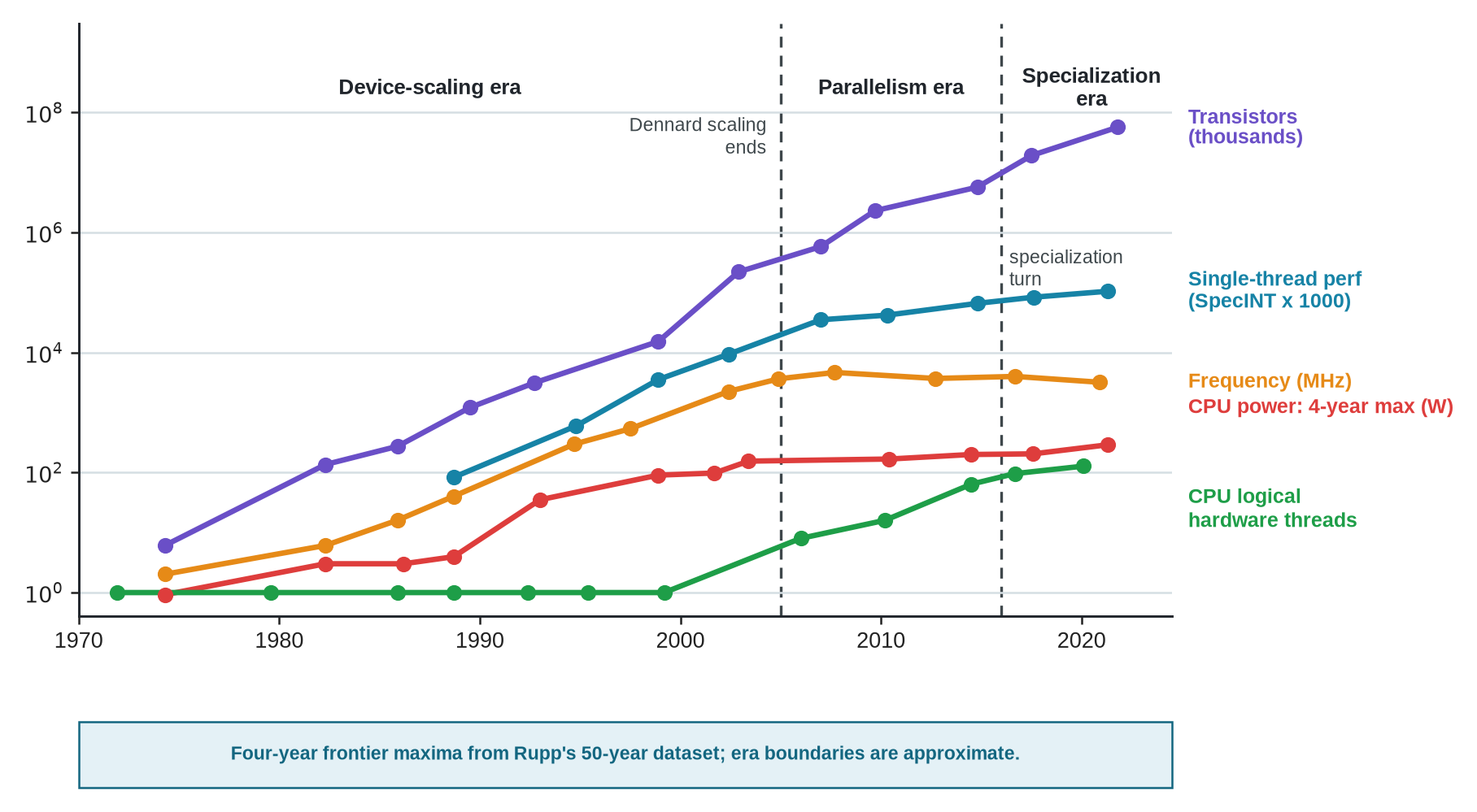
These diverging curves mark the conclusion of automatic hardware frequency scaling (Sutter 2005). Although transistor counts kept climbing, once Dennard scaling ended around 2005, the single-thread gains we historically associated with each generation slowed from roughly 50 percent a year to just a few percent (Hennessy and Patterson 2017). We must fit any further gains within the power envelope a package can dissipate. We also need to read the power trend carefully. The value near 300 W represents the highest entry in the final four-year interval of the public dataset, rather than a typical processor’s thermal design power. Like the other series, it highlights the frontier represented in the dataset so we can compare the directions of change on one chart.
Maintaining constant electrical properties during scaling depended on lowering voltage as transistor dimensions shrank (Dennard et al. 1974). Once voltage scaling slowed, power limits dictated how many transistors we could operate at full frequency at the same time (Esmaeilzadeh et al. 2011). This constraint helps explain both the frequency plateau in Figure 2.1 and the dark-silicon fraction that followed, the share of our chips that must remain inactive or unpowered to fit within a strict Thermal Design Power (TDP) budget. Our discipline responded increasingly with parallelism and domain specialization. These responses require us to manage more of the machine, rather than relying on automatic benefits from the next process node.
Although our measured history does not guarantee what comes next, technology continues to supply transistors without automatically turning them into proportional frequency or single-thread performance. These expanding design choices increase the workload that any new tools or assistance must help us improve.
2.2.2 Domain Specialization Tightens Cross-Layer Stack Coupling
Technology, architecture, workloads, compilers, and implementation were never truly independent. The layered stack remains a useful abstraction because it helps us separate different kinds of reasoning. Device technology supplies transistor characteristics, architecture organizes the machine, and the optimization layer covers the mapping, scheduling, and tuning that connect software to our hardware. Specialization does not create this coupling; instead, it tightens existing cross-layer dependencies.
The classical decoupled design stack and the modern specialization-coupled design loop differ in exactly one structural property, whether the layer boundaries stay independent (Figure 2.2). Domain specialization breaks the clean layer abstractions of the traditional vertical hierarchy: optimization, architecture, and technology become mutually dependent, bound together within shared power, thermal, and area limits. An accelerator decision made in software mapping or microarchitecture propagates immediately down to physical placement and thermal signoff, requiring us to evaluate software, architecture, and physical implementation as a single coupled system.
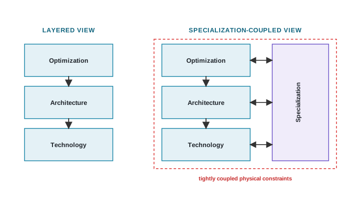
Our layered view keeps optimization, architecture, and technology distinct enough for us to reason about them separately. The specialization-coupled view retains that useful decomposition, but makes the two-way dependence explicit by enclosing our choices within shared power, thermal, and area limits. Consequently, specialization makes our workload mappings, architectural mechanisms, and physical implementations far more consequential to one another.
When we rely more heavily on caches, speculation, vector units, multicore processors, accelerators, and system-level optimization, we recover efficiency. However, every one of those choices introduced a new way for an early model to rank the wrong candidate. This comparison problem only compounds as we integrate those mechanisms into even larger systems.
2.3 Balancing Microarchitectural Scaling, Specialization, and Composition
As our designs evolve from a single core to a complete system, our methods of comparison must scale alongside them. Microarchitecture weaves intricate policies within a core, specialization binds a block to a specific workload, composition integrates diverse blocks into a single package, and wafer-scale integration stretches a unified fabric across new physical dimensions. Every step multiplies the parameters we can tune and the complex interactions our comparisons must account for.
2.3.1 Pipeline Depth, Issue-Window Complexity, and Speculative Corner Cases
Consider the familiar levers already in our architectural toolkit. Extending a pipeline, deploying a more aggressive branch predictor, widening a speculative scheduler, or scaling out the cache hierarchy can all recover performance.
However, each of these levers introduces corner cases that our benchmarks must carefully navigate. A prefetcher that anticipates one access pattern might pollute the cache for another. Increasing speculative execution can improve throughput, but it burns more energy and, as Spectre and Meltdown reminded us, can breach protection boundaries and leak speculative transient data (Kocher et al. 2019; Lipp et al. 2018). The gains we measure on one workload often obscure hidden costs that only surface elsewhere.
We have long known that these microarchitectural mechanisms hit fundamental physical limits. Palacharla et al. (1997) demonstrated that dynamic out-of-order execution cores face steep physical complexity bounds, where wakeup tag-drive delay grows quadratically with instruction window size \(N\) and bypass delay grows quadratically with issue width \(W\), while selection logic grows only logarithmically in \(N\). Wire delay on these critical paths eventually dominates the clock cycle, capping achievable frequency. Agarwal et al. (2000) subsequently projected that the combined impact of interconnect delay and clock scaling would ultimately conclude the frequency-first era for conventional microarchitectures.
These microarchitectural costs translate into concrete engineering realities. Intel’s Pentium 4, leveraging the NetBurst microarchitecture, stretched to 31 pipeline stages in its 90 nm Prescott generation (up from Willamette’s 20 stages) to chase aggressive 4 GHz frequency targets (Boggs et al. 2004). While deepening the pipeline reduces the logic depth per cycle, it penalizes branch mispredictions by inflating refill latency to over 30 cycles. When a branch predictor misses, the entire 31-stage pipeline drains, creating execution bubbles and burning dynamic power (\(P = C \cdot V^2 \cdot f\)) while Instruction Per Cycle (IPC) collapses on branch-heavy workloads. This classic example clarifies our central trade-off. Frequency is never an isolated design objective. The very mechanisms we use to push clock speeds alter the work required per instruction and the energy our machines consume.
Scaling out to multiple cores introduces an additional layer of complexity. Coherence protocols, memory-ordering rules, synchronization overheads, and workload partitioning all dictate how our designs behave in the wild, and none of these effects register in a single-threaded proxy metric. Even at this stage, before integrating a single specialized block, the volume of data required for a fair comparison has already outgrown any single summary number.
2.3.2 Specialization Traps and Amdahl’s Law
We should view specialization as a broad spectrum, not simply a binary leap from a general-purpose CPU to a custom accelerator. We can integrate vector and matrix execution units into standard cores, leverage GPUs for massive parallel execution, craft domain-specific accelerators with custom dataflows and memory hierarchies, or strip away flexibility entirely with fixed-function application-specific integrated circuits (ASICs). As we slide along this spectrum, we trade the breadth of workloads and software paths our hardware can run for raw efficiency.
This spectrum redefines what our comparisons must weigh. While microarchitecture and multicore scaling refine a general-purpose foundation, specialization bends the hardware around a specific workload. Consequently, we must shift our metrics and expand the design space we evaluate. A thermally constrained mobile chip sipping battery power and a warehouse-scale system choked by power delivery and total cost of ownership (TCO) disagree on what “efficiency” means. We can only fairly judge a specialized block against the specific target it was engineered for.
The potential upside is large. Across the computational kernels examined by Hameed et al. (2010), a bespoke fixed-function ASIC proved roughly 500 times more energy efficient than a conventional core. They captured most of this efficiency gain by eliminating instruction fetch, decoding, and redundant data movement, while simultaneously exploiting massive parallelism and fused operations. This result does not guarantee identical gains across the board. Instead, it highlights exactly why deciding what to specialize, determining which flexibility to keep, and shaping the software interface have become our central architectural challenges.
This drive for specialization has spawned a wide diversity of designs, a period the team behind Project Brainwave, Microsoft’s deep-learning acceleration platform, described as one of rapid architectural diversification (Chung et al. 2018).
For a sense of how expansive, Figure 2.3 plots roughly 180 publicly announced AI accelerators from the MIT Lincoln Laboratory survey (Reuther et al. 2025). They span seven orders of magnitude in peak power, from sub-watt embedded chips to multi-kilowatt data-center clusters, and six orders of magnitude in peak performance, from giga-operations to hundred-peta-operations per second, with energy-efficiency contours running from 100 GOps/W to 100 TOPS/W. Across form factors and across both training and inference roles, the parts form a dense, heterogeneous cloud rather than clustering around a single operating point.
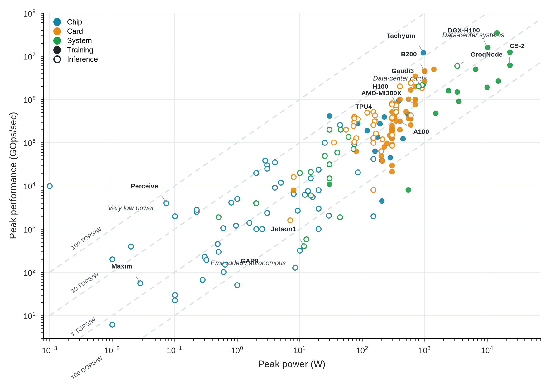
As architects, we have to decide precisely what to specialize, where that custom logic belongs, and how it will talk to the rest of the system. Choosing between a standard CPU and a custom accelerator is just our opening move. That initial pivot requires answering a series of subsequent architectural questions. What is our ideal vector length? How should we structure the memory hierarchy and local buffers? What dataflow, precision, and compression schemes make sense? How do we handle runtime scheduling, compiler support, strict deadlines, thermal throttling, and fallback modes?
In practice, specialization offloads the heaviest computational lifting to a heterogeneous cluster of Domain Specific Architectures (DSAs), leaving our general-purpose cores to handle control flow and the long tail of tasks that yield minimal acceleration benefit. We rarely find a universal partition; instead, the ideal balance shifts dramatically from one system to the next. Every new DSA we integrate threatens to drag in its own bespoke programming model, instruction set extension, or unwieldy toolchain obligation.
Specialization binds the value of our hardware directly to the efficiency of a targeted workload. Before we carve out die area for a specialized block, we must confront Amdahl’s law and ask what fraction of the deployed workload we are actually accelerating. If our targeted kernels only consume half the total execution time, an accelerator that executes them ten times faster will still yield a total speedup of about 1.8x, simply because the unaccelerated half now dominates the critical path (Amdahl 1967). The work we leave behind on the general-purpose core defines the ceiling of our specialized gains. Therefore, we cannot evaluate a specialized block in isolation; we must judge it alongside the compiler, the runtime, the memory traffic, and the residual workload that collectively determine its true delivered benefit.
2.3.3 Packaging and Chiplet Composition Risks
Specialized IP blocks rarely ship in isolation. We actively weave them into complex systems-on-chip (SoCs) and, increasingly, distribute them across multiple discrete chiplets. Manufacturing yield heavily drives this shift. Under classical random-defect models, die yield falls steeply with die area (Murphy 1964), so fracturing a large monolithic die into smaller compute and I/O chiplets recovers yield. However, this strategy does not linearize our costs, since advanced packaging, chiplet reuse, and heterogeneous process nodes completely rewrite the underlying economic model (Feng and Ma 2022). Beyond yield, chiplets allow us to freely mix process nodes, third-party IP blocks, and specialized memory arrays on a single substrate. Open standards like Universal Chiplet Interconnect Express (UCIe), an open die-to-die interconnect standard (UCIe Consortium 2026), stabilize the physical layer, with specification targets of sub-picojoule energy efficiency (\(<0.5\text{ pJ/bit}\)) and high shoreline bandwidth density (\(>1.3\text{ TB/s/mm}\)) across micro-bump pitches (\(25\text{--}55\,\mu\text{m}\)). Yet they leave the partitioning and implementation choices entirely in our hands.
These advantages demand that we navigate coupled design choices. A multi-chiplet system is far more volatile than just a miniaturized motherboard shoved into a package. Advanced packaging (such as 2.5D silicon interposers or 3D micro-bump arrays) alters our latency, bandwidth, and energy budgets while introducing severe thermal coupling and rigid physical constraints. A modern SoC also typically integrates heterogeneous IP blocks sourced from many different vendors.
In industrial practice, SoC projects frequently integrate new specialized blocks alongside legacy controllers and proprietary physical-interface IP without full RTL visibility. We must manage undocumented interface behaviors, conflicting reset sequences, and complex clock-domain crossing (CDC) constraints that resist simplified analytical modeling. Assembling the full system can uncover subtle coherence-protocol mismatches (Arm Limited 2020) or timing violations. Additionally, networks-on-chip (NoCs) can experience deadlock if cyclic dependencies enter the channel-dependency graph.1 These integration risks often remain undetected until late-stage verification or physical silicon bring-up.
1 Routing deadlocks: A routing function is deadlock-free when its channel-dependency graph has no cycles. Virtual channels can remove those cycles (Dally and Seitz 1987).
Each additional IP block integrated into a design restricts the space of valid configurations. Partitioning a function across a chiplet boundary alters the physical interfaces, shifts the software path, and requires different evaluation tools.
Heterogeneous modules also compete for shared interconnect resources. The network-on-chip (NoC) must arbitrate between high-throughput bursty accelerator traffic and latency-sensitive real-time traffic under strict deadlines. Average bandwidth estimates can obscure microarchitectural contention that causes latency violations.
When automating exploration across multi-component systems, search algorithms encounter two primary failure modes. If the search remains unconstrained, algorithms waste compute evaluating invalid configurations that violate physical feasibility. Conversely, overly restrictive constraints risk excluding viable candidate architectures. Before executing a search algorithm, we must define valid transformations, fixed interfaces, legal configurations, and evaluation budgets. Evaluating a large candidate count alone does not resolve these critical questions.
Across multi-vendor packages, formal specifications are often incomplete. The Semiconductor Research Corporation’s Microelectronics and Advanced Packaging Technologies (MAPT) roadmap notes that design automation for packaged multi-vendor systems is constrained by the absence of standardized data formats, syntax, and semantics across suppliers (Semiconductor Research Corporation 2023). Optimization algorithms cannot enforce an integration rule unless suppliers specify it in a machine-readable format.
System composition multiplies the physical and economic constraints candidate designs must satisfy. Long software bring-up sequences exceed the practical execution limits of detailed software simulators like gem5 (Binkert et al. 2011) or MacSIM (a heterogeneous many-core timing simulator), forcing teams to rely on hardware emulation or FPGA prototyping. Tools like FireSim (Karandikar et al. 2018) provide FPGA-accelerated full-system simulation to address this bottleneck. Yet each platform requires trade-offs between execution throughput, debug visibility, hardware cost, and environment setup complexity.
Beyond functional correctness, chiplet manufacturing, security, power integrity, and IP interfaces demand independent verification. In advanced 2.5D and 3D integration schemes, such as TSMC’s CoWoS (TSMC 2023) or Intel’s Foveros (Intel 2023), discovering a defective die after packaging renders the entire assembly non-functional. While pre-bond screening mitigates yield losses, it cannot guarantee that every die survives the physical stresses of packaging and assembly. Consequently, architectural partitioning must incorporate adequate test access and support pre-bond screening (such as IEEE 1838 test access architecture) to establish Known-Good-Die status.2
2 Known-Good-Die (KGD): KGD is the screening status assigned to a bare die judged suitable for assembly. Test-access work for three-dimensional stacks covers both pre-stacking die tests and post-stacking tests because screening one die does not establish the behavior of the completed assembly (Marinissen et al. 2010; IEEE 2020).
Security introduces additional constraints. Unsanitized sharing of speculative buffers or execution units across security domains introduces microarchitectural side-channel vulnerabilities. Validating these boundaries requires formal verification or penetration testing, as standard performance proxies cannot detect security flaws. High current densities in multi-chiplet packages likewise induce voltage droops, where package inductance \(L\) and rapid current transients \(\frac{di}{dt}\) create inductive supply noise (\(L \cdot \frac{di}{dt}\)) alongside static resistive IR drop. Layout signoff therefore requires detailed power delivery network (PDN) and thermomechanical modeling rather than aggregate power estimations. Additionally, IP blocks may lack internal visibility; for instance, Arm has supplied processor IP as fixed hard macros (Arm Limited 2013), and Intel distributes encrypted RTL (Intel Corporation 2024). In these scenarios, we have restricted access to internal state, increasing reliance on interface verification.
2.3.4 Wafer-Scale Fabrics and Communication Latency Bounds
Some systems demand more raw compute, memory capacity, or internal bandwidth than any conventional package can ever deliver within a practical power envelope. Wafer-scale integration answers this by extending the machine to a new physical scale, all while preserving the illusion of a single tightly coupled fabric (Pal et al. 2019). While large machine-learning accelerators make this breaking point visible today, we face the same architectural trade-offs far beyond the domain of AI workloads.
When we place dozens of compute and memory regions on a single wafer-scale fabric, we can reduce the communication overhead that would burden a board- or rack-scale network. However, this scale pulls power delivery, physical reach, manufacturing yield, routing, dynamic repair, thread scheduling, and data placement into a single, massive architectural comparison. In a wafer-scale GPU case study, physical constraints reduced usable capacity from a nominal 100 GPU modules to 40, requiring architects to co-design software scheduling and data placement alongside physical hardware (Pal et al. 2019).
Consequently, wafer-scale engineering introduces system-level constraints typically associated with rack-scale networks. Defective dies or interconnect failures require dynamic redundancy and rerouting, while physical communication distance and software mapping govern net usable capacity. Architectural comparisons must account for power delivery, communication overheads, defect repair limits, and software mapping rather than evaluating peak compute in isolation.
At every physical scale, from a single core out to an entire wafer, our delivered benefit hinges on software placement, dynamic scheduling, and an unbroken executable path. As we scale up, the next pressure we face is not designing yet another piece of hardware. Instead, we must confront the software stack required to keep the machine fed.
2.4 Software as Silicon
Hardware provides minimal utility without the compilers, runtimes, libraries, and applications that map a workload onto it. This dependency can fail in two directions. We gain nothing from a mechanism that no compiler can target, and we might see diminishing returns if we optimize against a software stack that later changes.
2.4.1 Executable Software Paths
Even after our hardware candidates clear physical constraints and evaluation budgets, our software must actually be able to use them. The executable software path encompasses the programming model or front end, compiler, libraries and kernels, runtime, driver or firmware, operating system, and deployment controls. We need all of these to exploit a hardware mechanism without losing its benefits to data movement or overhead. Historical shifts like RISC and CUDA succeeded precisely because they provided the compiler support and programming models that made the hardware accessible. Conversely, a design with high peak floating-point operations per second (FLOPS) will fail if we cannot use its software contract.
Consider the IBM/Sony/Toshiba Cell Broadband Engine, which required developers to manage local static random-access memory (SRAM) stores through explicit direct memory access (DMA) transfers (Kahle et al. 2005). This mechanism makes the software obligation concrete. When we compare designs, we must evaluate the code, scheduling, and data movement needed to use the local stores, rather than relying solely on the hardware’s peak throughput. When we build specialized hardware without a usable software path, we introduce hidden costs that peak hardware metrics never reveal.
We must treat a hardware proposal as incomplete until we can inspect and test the software path needed to use it. Modern tensor programs turn that path into a search problem of its own. Frameworks like Halide (a domain-specific language and compiler for image processing) and MLIR (a modular compiler infrastructure for multi-level intermediate representations) integrate scheduling, lowering, and intermediate representations directly into our performance comparisons (Ragan-Kelley et al. 2018; Lattner et al. 2020). If we rely solely on a hardware optimizer, we might select a mechanism that our compilers cannot target, or we might suffer software overheads that erase our predicted gains. To be credible, our comparisons must evaluate the entire executable hardware-software path, rather than examining a hardware block in isolation.
In principle, we can run a joint search that varies compiler schedules alongside hardware parameters, using a shared schema such as an MLIR dialect to co-generate the intermediate representation and the RTL. This approach might uncover combinations that we would miss in separate hardware and software studies, but we must test this hypothesis rather than assuming a guaranteed benefit. On the software side, we have already demonstrated search at enormous scale, as autotuners (such as AutoTVM, a machine learning-based tensor program optimizer (Chen et al. 2018)) search spaces of billions of tensor-program schedules. However, if we want to claim that we co-optimized the hardware and schedule to produce a better system, we still need an evaluation that scores both sides at matched fidelity. These evaluation gaps, rather than the search itself, are where our co-design efforts typically stall.
As we scale to distributed systems, our software path grows even more complex. Compiling code for a single node is no longer enough. Our execution path now relies on communication primitives such as the Message Passing Interface (MPI) and NVIDIA Collective Communications Library (NCCL), alongside systems that coordinate computation across many accelerators. For example, Alpa, an automated framework for inter- and intra-operator parallel execution (Zheng et al. 2022), automatically derives parallel execution plans for distributed deep learning, while Megatron-LM, a large-scale transformer training framework (Narayanan et al. 2021), combines tensor, pipeline, and data parallelism. Our choices in collective selection, topology awareness, and runtime scheduling dictate whether thousands of accelerators can actually deliver the throughput we predicted for a single device.
We should view the instruction set architecture (ISA) as just one boundary within a much larger software path. Whenever we introduce a new vector or accelerator interface, we must preserve the relevant application binary interface, memory model, operating-system assumptions, compiler lowering, runtime behavior, and compatibility tests. We also need our compiled programs to demonstrate that data movement and software overheads do not consume our predicted benefits. We must not advance a design based on a favorable hardware proxy if we cannot compile, schedule, and test it. Establishing an executable path once does not freeze it for the life of the hardware. In many of our modern comparisons, proposing another hardware mechanism is no longer the limiting factor. Instead, our real challenge is re-establishing an executable, representative comparison every time our compilers, runtimes, libraries, workloads, or deployment policies change. This software path often evolves while we are still designing the hardware.
2.4.2 Software Speed vs. Silicon
Our software and workloads constantly evolve while we design hardware. Consequently, our architectural comparisons can become stale long before the silicon ships, even if the hardware design remains entirely unchanged.
Several parts of our target can shift during this interval. We regularly see changes in AI models, precision formats, sparsity patterns, compiler passes, kernel libraries, runtimes, serving systems, batching strategies, fleet policies, and benchmarks. For instance, precision formats like 8-bit floating point (FP8), 4-bit integer (INT4), and block-scale formats evolve rapidly, yet we must eventually fix our supported data types in hardware.3
3 Block-scale formats: Low-precision number formats amortize shared exponent or scale metadata across a block of elements rather than storing independent metadata for every element (Rouhani et al. 2023). Committing to one in silicon fixes our datapath choices even as formats and workloads continue to evolve, so we must carefully judge whether the choice will remain useful over time.
Every hardware decision encounters two kinds of software change, and our comparisons must explicitly state which one we are addressing. Before release, our hardware and software teams can revise the design together, though these late changes become increasingly expensive. After release, the hardware is fixed, but our compilers, kernels, libraries, runtimes, and deployment policies keep improving. These continuous improvements reveal performance that our initial evaluations never captured. If we want to claim post-release gains, we need clearly paired hardware, workload, and software versions, as we develop in Chapter 9. We also must separate the software improvements explicitly made for our hardware from unrelated shifts in the broader workload. The former strengthens our case for the existing design; the latter renders our original evidence stale.
Our primary challenge lies in determining whether a software change invalidates an architectural comparison or leaves it intact. Simply detecting that two traces or software versions differ does not answer this question. We must identify which specific differences could reverse our design decisions and determine which measurements will test that possibility.
While specialization can improve efficiency, it also makes our designs far less tolerant of workload drift. Conversely, generality preserves our flexibility, but often at a steep cost in performance per watt. As a result, we must bound the workload, continuously measure how it changes, and proactively revisit our hardware decisions whenever the original assumptions no longer hold.
We can see one bounded example of this in AI workloads, where model scale and computational demands shift visibly. While convolutional inference with fixed shapes tends to be regular, we often see dynamic behavior in autoregressive Transformer deployments due to growing key-value caches (W. Kwon et al. 2023), variable sequence lengths, sparse mixture-of-experts4 routing, or distinct prefill and decode phases (Agrawal et al. 2024). We recognize these as common sources of changing memory behavior, rather than universal properties of every model. To illustrate this rapid evolution, an Epoch AI report estimated a four- to fivefold annual growth in training compute for recent notable and frontier models through May 2024 (Sevilla and Roldán 2024). In Figure 2.4, we present a separate fit using the displayed records from a frozen July 19, 2026 snapshot of Epoch AI’s model database (Epoch AI 2025). We calculated a roughly 4.4-fold rate as our own fit to that snapshot, distinct from the original report. Both results depend heavily on model class, outliers, and our chosen form of fit. While compute growth itself is not workload drift, it illustrates why we cannot transfer evidence tied to one model scale, software stack, or training regime to another without explicitly checking our assumptions. A useful comparison must state which model, compiler, runtime, benchmark, trace, and deployment versions support each architectural decision.
4 Mixture-of-experts (MoE) routing: A sparsely gated model activates only a subset of its expert subnetworks for each input (Shazeer et al. 2017). Because this input-dependent routing forces memory traffic to vary from token to token instead of following one fixed schedule, we must design our hardware to serve highly dynamic memory demands.
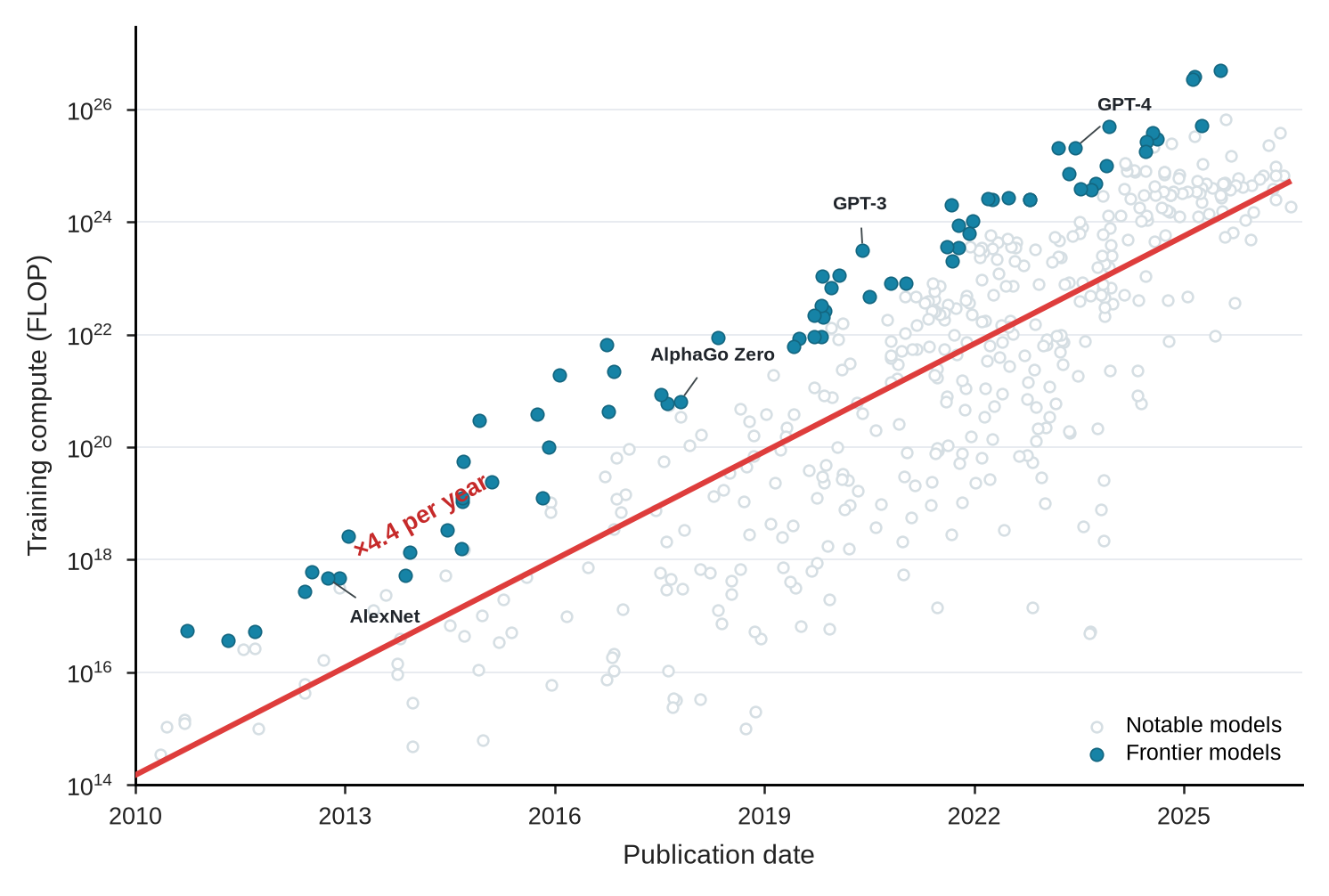
The notable-model and frontier records rise by orders of magnitude over the 2010–2026 window, and our fitted line summarizes that scattered cloud as more than fourfold annual growth. We do not use this fit to establish a universal rate, and we know that a larger model does not automatically constitute a different workload. Instead, it provides us with a bounded example of how rapidly model scale and the software stack can evolve while a hardware project is still underway. The specific model we sized our comparison against may ultimately differ from the model that eventually runs in production. For this reason, we must record the software and model versions behind our comparisons rather than taking them for granted.
Product announcements reveal intervals between commercial releases, not the period during which an architecture decision remains exposed to software change. The timeline compares those public intervals for two product categories relative to November 2020 (Figure 2.5). Apple client SoCs appear at 7- to 19-month intervals in this sample, while NVIDIA data-center accelerators appear at 22- to 24-month intervals. These dates motivate the versioning question, but they do not reveal either company’s internal design schedule or establish how long a hardware decision remained fixed.
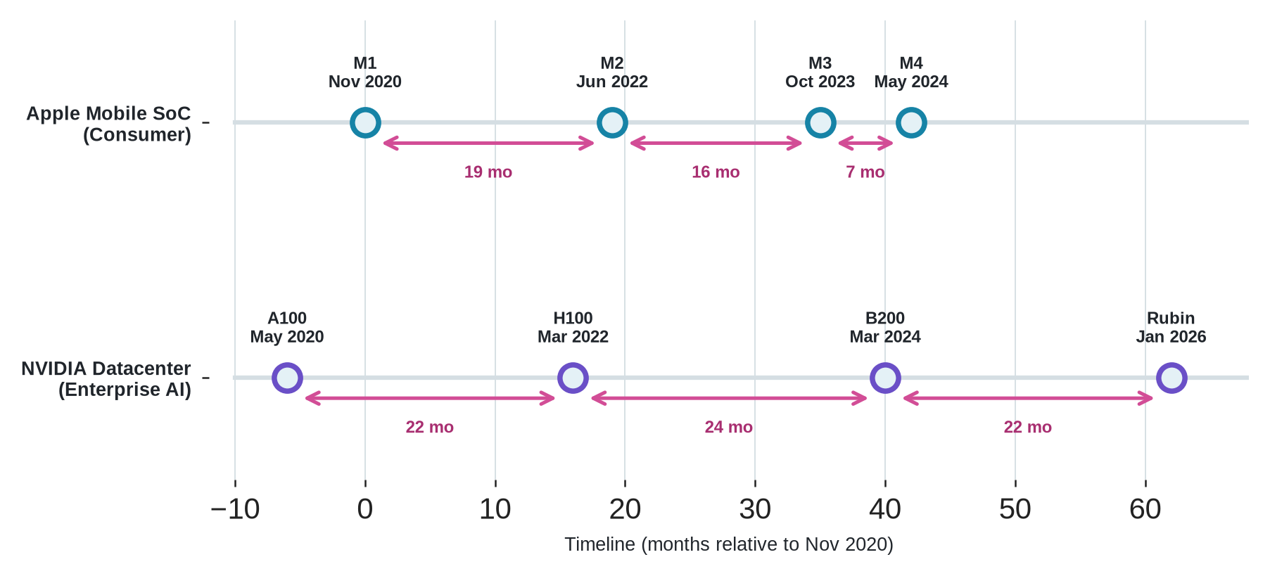
Apple’s gaps shrink rapidly from 19 to 16 to 7 months, while NVIDIA’s data-center GPU gaps remain near two years, at 22 and 24 months (Figure 2.5). We cannot use these announcement dates to bound a silicon program or to identify exactly when an architecture choice became too hard to change. They do not measure the pace of software change, rank release strategies, isolate any specific architecture contribution, or prove that AI tools caused a release to arrive sooner. Neither plot establishes a definitive design-cycle mismatch. Together, they illustrate why our comparisons must record the actual hardware, workload, and software exposure, rather than attempting to infer these details from public release dates.
We often use benchmarks to keep our changing workloads comparable. For example, MLPerf, an industry-standard machine learning benchmarking suite (Mattson et al. 2020), defines shared tasks and reporting rules for machine-learning systems. Within the same benchmark version, division, scenario, and accuracy target, its strict inference rules allow us to compare results from different systems (Reddi et al. 2020), all while giving submitters the freedom to optimize their software toolchains (Reddi et al. 2021). However, this comparability is actively maintained rather than inherent to the workloads themselves. The comparison only holds true as long as our community actively maintains the tasks and run rules.5 Whenever those underlying rules change, we may find that an earlier comparison no longer answers the same question.
5 Metrological traceability: A measurement result is traceable when we can relate it to a reference through a documented, unbroken chain of calibrations, each contributing uncertainty (Possolo et al. 2021). While our architecture benchmarks do not create this kind of formal calibration chain, we still need explicit versions for their tasks, run rules, and measurement procedures so that reviewers can verify when two results remain genuinely comparable.
For a target like Lighthouse mobile extended-reality (XR), the term “XR” remains far too broad to define a concrete workload, as it combines complex sensing, perception, graphics, display, interaction, latency, quality-of-experience, and energy constraints into a single concept. Five workload archetypes make the ambiguity concrete (ResNet-50 vision, GPT-2/Llama language models, DLRM recommendation engines, MobileNetV2 mobile perception, and KWS always-on keyword spotters), each pulling a design toward different memory, latency, and energy behavior. Even when we employ a dedicated benchmark suite like XRBench (H. Kwon et al. 2023), we must still independently decide which specific traces, model versions, deadlines, input distributions, and quality targets truly matter for our design.
We must therefore treat our workload description as a precisely versioned input rather than a static name. When we document versioned traces, benchmark rules, compiler and runtime assumptions, and tool results, we allow our reviewers to independently verify whether a hardware claim still holds true. Our architecture studies also need explicit triggers that prompt us to repeat the comparison the moment one of those inputs changes. When our machines span an entire data center, the executable software path dictates exactly how our hardware, networks, and facility resources successfully operate as a single, unified system.
2.5 Machine Boundary Expansion
Warehouse scale pulls all our preceding hardware and software pressures into a single architecture problem. Our server and accelerator choices no longer exist in a vacuum; they ripple outward through network topology, collective communication, cluster scheduling, failure handling, deployment policies, and even facility power and cooling. When we compare systems at this level, we must judge the delivered service and operating constraints of the entire infrastructure, rather than just admiring the efficiency of an isolated node.
Even if a single user request fits perfectly on one package, our aggregate demand, availability targets, and stringent service objectives often force us to deploy thousands of nodes. The boundary of “the computer” expands until it swallows the entire data center. As we adopt scale-out networks, sophisticated cluster software, and coherent device and memory interconnects like CXL (Compute Express Link), resource placement and sharing turn into fundamental architectural questions.6 We have officially entered the domain of warehouse-scale computing (WSC) (Barroso et al. 2019). Our architectural problem now encompasses everything from heterogeneous servers and shared cooling infrastructure to facility power limits and cluster-wide scheduling.
6 Compute Express Link (CXL): A cache-coherent interconnect standard for processors, accelerators, and memory devices. Its memory semantics and switching support allow us to treat device-attached or pooled memory as a system-level provisioning decision (Compute Express Link Consortium 2026).
Experimenting with or simulating warehouse-scale systems is challenging, largely because component failure is a constant reality rather than an exceptional case (Barroso et al. 2019). As architects, we must synthesize evidence by combining trace-driven and discrete-event models, emulation, controlled deployments, and raw production measurements. Yet, every model and measurement inevitably leaves something out. A simple trace might entirely miss the dynamic network congestion that drives high “tail at scale” latency (Dean and Barroso 2013). Similarly, a node that appears highly efficient in isolation can lose its advantage when delayed by stragglers or heavy distributed coordination. Our core challenge is selecting evidence at an affordable scale without oversimplifying the model in ways that remove essential system behaviors.
As we traverse these scales, we never get a clean slate; our architecture comparisons do not reset just because the system boundary expands. A single core contributes baseline policies and tricky corner cases. An accelerator brings along its own workload mapping and software interfaces. SoCs and chiplets add strict integration, packaging, and testing constraints. When we step up to wafer-scale and warehouse-scale systems, we inherit all those previous obligations while stacking on new burdens like repair, placement, networking, failure handling, deployment logistics, and facility limits.
This system boundary expansion steadily accumulates comparison obligations across five architectural scales, from a single core through accelerators, systems-on-chip (SoCs) and chiplets, wafer-scale systems, and warehouse-scale systems (Figure 2.6). As we expand system boundaries, the early microarchitectural and ISA obligations never disappear: each scale adds new evaluation obligations while carrying forward the constraints, interfaces, software paths, tool feedback, failures, and rejected alternatives established at smaller scales. A warehouse-scale evaluation must preserve core-level software correctness and chiplet-level physical constraints while absorbing cluster networking and thermal limits.
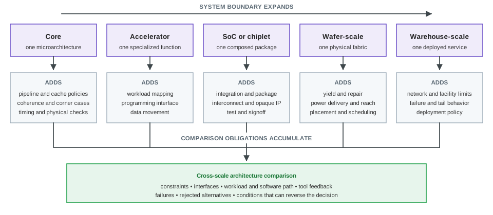
This progression is cumulative, though we are not claiming every architectural study must simulate an entire data center. If we are comparing cores, we might legitimately stop after our microarchitecture and physical checks. But a warehouse-scale comparison cannot stop there; our node’s behavior only reaches the delivered service through thick layers of software, complex networks, deployment policies, and rigid facility constraints. The appropriate boundary for our study is always the smallest one that captures the effects capable of flipping our final decision. Once we pull hardware, software, network, and facility choices into a single comparison, the number of possible combinations explodes far faster than our capacity to evaluate them.
2.6 Search Space Explosion
We must treat our capacity to produce candidate designs and our capacity to evaluate them as distinct resources. A mismatch often appears when hardware and software coupling expands the set of designs we can generate, yet our ability to check those designs fails to keep pace. We can easily conflate these two quantities simply because counting candidate production is much easier.
Even a narrow comparison can yield a large number of combinations. Let us look at some illustrative rather than measured arithmetic. Suppose we explore an accelerator and memory subsystem for our Lighthouse prompt, sweeping six of its stack layers while holding the rest fixed. If we consider five compute organizations (such as a vector-capable CPU, an accelerator, or an SoC block), four ISA and ABI contract options (such as RV64GCV vector extensions), six memory hierarchy and data movement topologies (such as NoC bisection bandwidth and DRAM timing choices), four power envelope targets (scaled around the 3 W TDP), three compiler and runtime stack paths (Triton, an open-source GPU compiler language, LLVM/MLIR, domain libraries), and three physical process libraries (such as TSMC N7 or a 3 nm-class LP mobile process), we obtain the following product.
\[ 5 \times 4 \times 6 \times 4 \times 3 \times 3 \]
We face 4,320 candidate configurations before we even begin counting workload versions, process corners, thermal constraints, or reliability cases. If we check each candidate at three fidelity levels, we create 12,960 candidate-evaluation combinations, all before we reject a single invalid design. In our real architecture studies, these numbers grow far larger and the process takes far longer before we ever see silicon measurements.
However, this raw count tells us little about how many candidates we can actually evaluate well enough to matter. Because each surviving configuration requires an analytical model, simulator run, synthesis check, or human review, our larger choice set dramatically increases the demand for feedback. We know that cheap models reduce evaluation cost, but they cannot establish whether a choice is truly legal or whether stronger measurements will preserve its ranking. Our practical limit is not how many configurations we can enumerate in an architecture study. Rather, it is how many we can evaluate rigorously enough to support our next design decision.
Four representative architecture tasks anchor how search space scale varies across hardware and software design domains (Table 2.2). Candidate space volume does not measure evaluation work or decision confidence, because validity constraints and simulation fidelity differ radically between mapping, accelerator Design Space Exploration (DSE), floorplanning, and compiler tuning.
When we look at Timeloop (Parashar et al. 2019), an analytical framework for mapping and evaluating deep-neural-network (DNN) accelerators, we find a concrete lower bound on this combinatorial growth. For a convolutional neural network (CNN) layer with seven nested loops and a four-level memory hierarchy, our loop ordering and level-bypass choices alone produce \((7!)^4 \times (2^4)^3\) arrangements. The first factor gives us a different ordering of the seven loops at each of our four memory levels. The second factor gives us a binary bypass choice at those four levels for each of three data spaces. Our factorization choices enlarge this mapspace even further. This formula, therefore, represents neither the complete count nor a count of useful mappings. It simply isolates two sources of growth before our legality, capacity, and performance constraints step in to remove most of the candidates.
| Architecture task | Scale anchor | Why candidate count is not enough |
|---|---|---|
| DNN accelerator mapping | Timeloop enumerates loop permutations, factorization choices, and level-bypass alternatives (Parashar et al. 2019). | Mapping is itself a combinatorial problem; architecture evaluation depends on the mapper and its constraints. |
| DNN accelerator DSE | MAESTRO, an analytical cost model for estimating DNN dataflow performance, reports 480M candidates, 2.5M valid designs, and 0.17M designs/s (H. Kwon et al. 2019). | Pruning rules determine which candidates are evaluated and which are never seen. |
| TPU-block floorplanning | The AlphaChip paper (describing Google’s reinforcement-learning layout generation engine) reported reducing placement generation from months of human effort to hours of machine time (Mirhoseini et al. 2021). | Routed physical quality and strong baselines still require separate evaluation. |
| Tensor-program tuning | AutoTVM, a machine learning-based tensor program optimizer, describes tensor-operator search spaces on the order of billions of possible implementations for a single GPU operator (Chen et al. 2018). | Compiler schedules create a hardware-dependent search problem of their own. |
We see candidate scale emerging from entirely different parts of the system. While Timeloop and MAESTRO show us just how quickly our mapping and accelerator choices multiply, AutoTVM reminds us that our software schedule can create a large search space even after we have locked in our hardware. Our floorplanning example exposes the other limit. Just because we can produce a candidate quickly does not mean we have established its routed quality.
MAESTRO makes this distinction especially clear. When we process 0.17M designs per second, we can examine its full 480M-candidate space in under an hour. In this scenario, we have access to plentiful, cheap analytical feedback. Our most difficult decision then becomes figuring out which apparent winners justify a more expensive evaluation.
The four scale anchors land fifteen orders of magnitude apart when their candidate space sizes share one logarithmic scale (Figure 2.7). They run from our toy SoC design space (\(4.3 \times 10^3\)) through MAESTRO accelerator DSE (\(4.8 \times 10^8\)) and AutoTVM tensor programs (\(\sim 10^9\), an order-of-magnitude estimate) to Timeloop’s loop-ordering and bypass lower bound (\(2.6 \times 10^{18}\)). Candidate space volume does not measure evaluation cost or evidence strength: a massive search space evaluated with analytical proxies may cost far less total compute than a small space evaluated through full gate-level timing signoff.
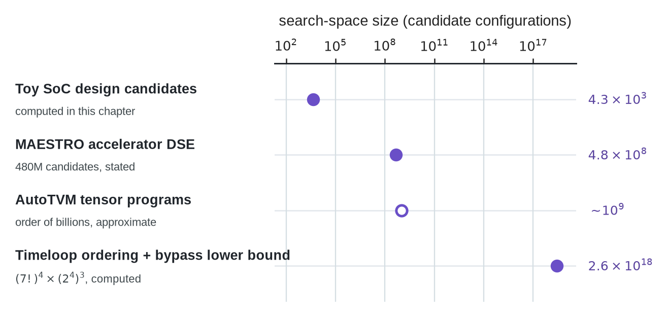
The toy count sits in the thousands, MAESTRO and AutoTVM cluster near \(10^9\), and Timeloop’s computed lower bound lies almost ten orders of magnitude beyond them (Figure 2.7). Yet this near-fifteen-order span encodes only candidate count; it tells us nothing about the cost, fidelity, or decision strength of a single evaluation. As architects, we must decide which choices are worth testing and how many reliable evaluations our architecture study can afford.
Our search capacity and evaluation capacity draw from completely separate budgets. ArchGym, an open-source machine learning gym for architecture design space exploration (Krishnan et al. 2023), clearly shows us why our exploration methods require fair, reproducible comparisons under common environments and shared sample budgets. Throughout this book, we apply an even broader accounting rule. We compare evaluation fidelity, tool cost, total compute, and engineering effort, rather than simply equalizing candidate counts alone. Although a fast estimator can increase the number of candidates receiving a quick score, it does not increase the number of candidates receiving a check strong enough to support our final commitment.
While broad search spaces and executable software paths provide the foundation for candidate generation, they still fail to establish how many configuration choices we can check strongly enough to support a robust decision. Our next real limit is the actual capacity, physical accuracy, and fidelity of our evaluation and verification pipeline.
2.7 Physical Limits and Throughput
We can keep growing our design space, but physics, budgets, and schedules still bound our comparisons. Physics dictates what we can actually build, power, and cool, while fixed program budgets and schedules dictate how much we can check before we commit to a tapeout. Though more resources might expand our evaluation capacity, they never remove underlying physical limits nor make our available time and money unbounded.
2.7.1 Physical Constraints
When we compare architectures, physical effects introduce two distinct problems. First, our early models might omit an effect that later overturns our initial rankings. Second, the definitive measurements that would settle the question often cost too much to run on every candidate. Consequently, a design that looks sound at our architectural abstraction can still fail due to a thermal hotspot or severe IR drop, revealing that our comparison masked a consequential physical effect. Reliability narrows the viable space further. Phenomena like soft errors, process variation (Borkar 2005), and silicon aging, including Negative Bias Temperature Instability (NBTI) and Hot Carrier Injection (HCI), directly affect viability in demanding domains like automotive systems governed by ISO 26262 (International Organization for Standardization 2018). To build confidence, we must often look to evidence from fault injection, aging simulation, physical and circuit analysis, accelerated testing, and production data.
Consider data movement, for example, which can reverse an early ranking based purely on compute. As we move data through a memory hierarchy, we often consume far more energy than we do performing arithmetic operations. Horowitz (2014) provides widely used estimates that quantify this difference. If we rely on a compute-only comparison, we risk ranking the wrong design first. Our results depend on where the data resides, how often it moves, who schedules it, what locality we can exploit, which precision we find acceptable, and what our software stack can express.
To quantify this physical reality, Figure 2.8 reports energy consumption per operation across arithmetic units and memory hierarchy levels using the 45 nm reference values from Horowitz (2014). A baseline 32-bit integer addition costs about \(0.1\,\text{pJ}\) (\(1\times\)); floating-point arithmetic runs \(0.9\text{--}4\,\text{pJ}\) (\(9\text{--}40\times\)); 8 KB to 32 KB SRAM cache reads run \(10\text{--}20\,\text{pJ}\) (\(100\text{--}200\times\)); a 1 MB on-chip SRAM access costs \(100\,\text{pJ}\) (\(1000\times\)); and off-chip DRAM accesses reach \(1.3\text{--}2.6\,\text{nJ}\) (\(13{,}000\text{--}26{,}000\times\)). Fetching data from off-chip DRAM thus consumes thousands of times more energy than performing arithmetic on that data, so an architectural comparison that omits memory hierarchy and locality can rank the wrong design first.
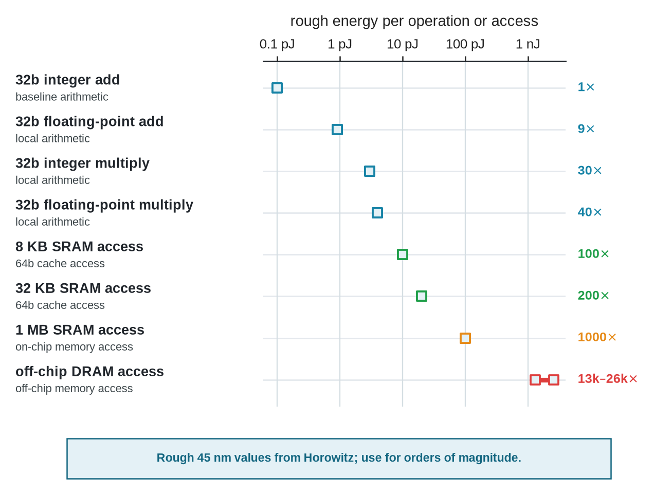
The DRAM cost is a range rather than a single point, and the values are order-of-magnitude anchors relative to the 32-bit integer addition: advanced nodes change the exact numbers, but the locality argument still holds rather than acting as a current-node energy estimate (Figure 2.8). It reminds us that we must model our memory hierarchy before we rank candidates.
We use a structural architecture-level energy breakdown. \[ E_{\mathrm{system}} = E_{\mathrm{compute}} + E_{\mathrm{memory}} + E_{\mathrm{interconnect}} + E_{\mathrm{control}} + E_{\mathrm{leakage}} \tag{2.1}\]
We intend this as a structural breakdown, not a rigorous circuit-level energy model, and it delivers a clear lesson in diminishing returns. In Equation 2.1, this decomposition directly reflects two persistent physical limits. First, the memory wall identified by Wulf and McKee (1995) highlights that logic performance scaling continuously outpaces DRAM access latency improvements, elevating off-chip memory access into the primary latency and energy bottleneck. Second, as multi-core and accelerator tile counts scale, Network-on-Chip (NoC) bisection bandwidth contention becomes a governing throughput bottleneck. High inter-tile communication and memory traffic saturate physical wiring and router buffers across die bisection cuts, causing routing congestion and severe backpressure. If an optimization focuses solely on compute efficiency while ignoring memory hierarchy and interconnect topology, unoptimized data movement and leakage terms quickly dominate system energy and render the design physically infeasible.
The proxy-mismatch failure shows up directly when we compare total system energy between a balanced baseline design and an unoptimized accelerator candidate (Figure 2.9). The candidate shrinks compute energy (\(E_{\mathrm{compute}}\)), yet its added memory accesses and communication overhead swell memory and interconnect energy (\(E_{\mathrm{memory}} + E_{\mathrm{interconnect}}\)) enough to push the system total above the baseline. Reducing compute energy in isolation can thus increase data movement and interconnect energy, inflating total system energy and causing partial evaluation metrics to rank an inferior design first.
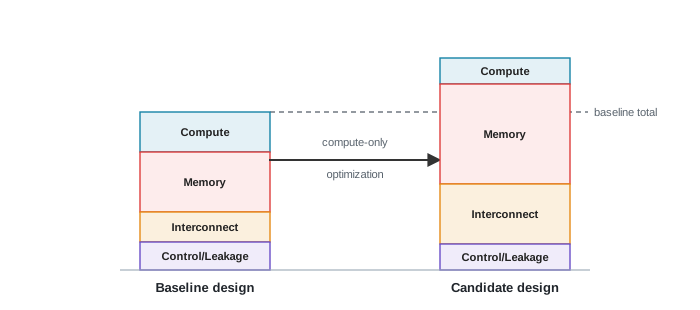
The numbers here are illustrative, but the reversal in Figure 2.9 is exactly our point: an early proxy might strongly favor a design that ultimately loses once we properly account for the costs of moving data through the system. We explore this specific proxy-mismatch failure directly in Chapter 7.
We must give interconnect costs the same rigorous attention as memory movement. Our on-chip networks, package links, memory interfaces, collective operations, and host-device protocols limit what our designs can sustain. During early logical synthesis and architectural modeling, we rely on approximate interconnect estimates, whereas detailed placement and routing expose our actual topology, congestion, and parasitic delays (Kahng et al. 2011). Because of this gap, a highly parallel accelerator might score well in our early models, only to fail timing or routing during physical implementation. The fundamental failure here is not that our early tools completely ignore wires; rather, it is that a clever optimizer will always exploit whatever our inexpensive models leave out.
Because timing, placement, routing, IR drop, thermal behavior, power delivery, leakage, signoff, and test requirements can easily overturn an architectural choice, we must consider relevant electronic design automation (EDA) and physical-design constraints as early as possible. These deep physical checks rely heavily on stateful tools, meaning a repeated run becomes entirely invalid if stale constraints or cached netlists survive from a previous candidate. While Chapter 6 covers our detailed tool isolation and execution mechanics, our core point here is that a clean tool state remains an absolute prerequisite for a valid comparison. For example, local power and thermal density can flag a dense accelerator mapping as highly risky long before implementation, even if its average power comfortably clears an early limit.
Once we have a placed netlist and a current profile, fast learned IR-drop estimation (Xie et al. 2020) and authoritative thermal signoff can either confirm or clear that risk. Thermal Design Power (TDP), which serves as a target for sizing our cooling solution rather than a strict measure of sustained power draw, is not our only limit (Intel Corporation 2014). For instance, rapid clock-gating transitions or 512-bit SIMD vector lane wakeups induce severe step-current transients (\(di/dt\)), causing localized \(L \cdot \frac{di}{dt}\) voltage droops on the power grid that force conservative frequency guardbanding or dedicated Emergency Voltage Mitigation (EVM) circuits. If we employ early physical estimates, workload-aware power models, and closer coordination between our microarchitecture and physical design, we can expose these subtle risks long before final signoff.
Vector execution makes the policy interaction concrete. When we add 512-bit vector units to general-purpose CPU cores, we raise our peak floating-point throughput. However, sustained wide-vector execution might raise power and power-delivery demand enough to force the processor to reduce its operating frequency. Peak vector width alone does not determine our final application speed; as architects, we must carefully measure the active-frequency policy alongside our exact mix of vector and nonvector work on the target processor.
During timing signoff, we evaluate multiple analysis views that pair operating modes with specific process corners using static timing signoff tools like Cadence Tempus (Cadence Design Systems 2021). We often find that our design might clear one view but completely fail another. Because our physical-design tools rely on heuristic optimization, a single failed closure attempt rarely tells us whether our candidate or a flawed tool setup caused the failure. When we carefully compare constraints, seeds, and repeated outcomes, we can better separate true design flaws from tool artifacts.
Design Rule Checks (DRC) introduce yet another rigorous physical constraint. Our routing must satisfy restricted design rules, including stringent minimum wire and via spacing (Kahng et al. 2011). Simply moving a single macro can spawn numerous violations, and repairing just one can alter neighboring routes and expose fresh errors. If our automated flow cannot interpret these markers intelligently, we dump a large, repetitive cleanup and rerouting burden onto our implementation team.
Artifact-producing flows introduce a traceability problem of their own. If our high-level tool emits RTL and a physical-design tool reports a thermal failure much later, tracing that failure back to the specific architectural decision that caused it becomes difficult. Since we can often rerun a saved RTL or topology artifact for deeper inspection, our design team must preserve the emitted artifacts, parameters, and tool states rather than hoping we can somehow recreate them later. When we evaluate these physical constraints, we also face the challenge of bridging the deep semantic gap between our high-level proposals and intricate EDA formats like LEF/DEF and Liberty timing files.7
7 LEF/DEF and Liberty: In our place-and-route flows, LEF carries the abstract physical information we use to place and connect blocks, while DEF captures the fully placed and routed state of our specific design (Silicon Integration Initiative n.d.). Meanwhile, Liberty provides characterized cell models covering timing, power, noise, and related behaviors (Synopsys 2012). We rely on these implementation formats to expose the essential details missing from our high-level architectural descriptions.
To manage this complexity, we increasingly turn to multifidelity methods that pair abundant, inexpensive estimates with carefully selected high-fidelity evaluations. We retain the stronger model to repeatedly check the accuracy of our proxy, a strategy familiar across engineering optimization, not just architecture (Peherstorfer et al. 2018). Our physical constraints demand exactly this level of care. If we know our early model omits timing, congestion, thermal behavior, or data movement, we must secure a more robust model before we confidently compare more candidates.
While an inexpensive energy proxy can support our early screening efforts, our finalists require an accurate, current power model before we can make binding power or efficiency decisions. We encounter this same limitation when measuring whatever metric we happen to be optimizing. A design can easily lead on the figures advertised in a standard data sheet, yet still fall behind on the actual work a real program executes.
The evolution of AMD’s Bulldozer architecture, its later FX-9590 product, and the subsequent Zen transition illustrates this gap between easy-to-count specifications and real-world workload behavior (Butler et al. 2011; Advanced Micro Devices 2014, 2017).
War story: A design that won on the spec sheet
The gap. Unfortunately, those figures did not reflect how real workloads actually used the machine. The shared structures became performance bottlenecks when threads competed for resources, and raising clock frequencies increased power draw. AMD’s later FX-9590 specification listed a high 220 W thermal design power.
The lesson. Candidates must always be ranked on the metrics their true workloads reward, rather than the numbers that are easiest to count. In silicon, discovering that gap is expensive, because it only becomes undeniable after the design is shipped. AMD eventually addressed this by introducing the Zen microarchitecture, returning to a renewed, disciplined emphasis on core performance and efficiency.
Because physical constraints and reliability concerns define a vast search space, no early model will ever eliminate our need for the robust physical tools required to validate our final claims. As architects, we must understand which lower-cost estimates are safe for broad screening, and which rigorous checks retain the power to overturn our rankings.
2.7.2 Simulation Throughput and Fidelity
As we design larger systems, we expose vastly more candidate configurations, software states, physical corners, and failure modes. Expanding our choice space inherently drives up our demand for simulator runs, synthesis runs, physical-design tools, verification passes, and expert review. We simply cannot run every candidate through every available tool. Since these evaluations consume varying mixtures of compute clusters, software licenses, project schedule, and human attention, our feedback loop starves whenever an architectural study demands more checking capacity than our available people and tools can provide.
Our evaluation tools form a broad spectrum where adjacent tiers often sit orders of magnitude apart in throughput, cost, and setup time. Suppose, as an illustrative working rate, that a detailed simulator like gem5 sustains ten to one hundred thousand instructions per second. At those rates, simulating just one real-time second of a workload retiring one billion instructions per second takes \(10^{9}/10^{5}\) to \(10^{9}/10^{4}\) host seconds, roughly three to twenty-eight hours. Fast parallel simulators like Sniper or compiled C++ RTL models generated via Verilator run significantly faster, while hardware emulation platforms (such as Cadence Palladium, an enterprise hardware emulation system, or Synopsys ZeBu, a high-throughput emulation engine) and FPGA prototypes (like FireSim, an FPGA-accelerated full-system simulation platform (Karandikar et al. 2018)) accelerate execution even further. Yet, each step up the fidelity spectrum demands different hardware, complex logic synthesis (via open-source engines like Yosys or industrial suites), and substantial bring-up costs. Since actual rates always depend on the model, workload, host, tool, and platform, our budgeting question is not just whether a candidate can be measured, but rather which candidates have actually earned the right to consume an expensive evaluation tier.
To cope, we have long rationed our expensive evaluations through abstraction and statistical sampling. For example, SimPoint, a profile-driven simulation sampling framework (Sherwood et al. 2002), helps us isolate representative program regions, while SMARTS, a statistically rigorous sampling methodology (Wunderlich et al. 2003), gives us rigorous error bounds for sampled simulation. We employ analytical models, reduced workloads, and multifidelity evaluation to serve this exact same purpose across different design levels. Because every one of these techniques trades some fidelity for capacity, we must clearly state what our cheaper evaluations preserve and explicitly flag which candidates still mandate a stronger check.
Making this allocation decision is difficult. While generating or scoring one more candidate might feel cheap, an inaccurate screening tool can discard a breakthrough design or advance a weak one into our most expensive stages. We have to decide which inexpensive checks can safely reject a candidate, which nagging uncertainties demand stronger tools, and which measurements are most likely to completely flip our final decision. If we fail to make these distinctions, generating candidates faster merely dumps more unproductive work into our design program’s most expensive, back-end stages.
The substantial costs of leading-edge chip development illustrate the magnitude of this constraint. Although public estimates vary and should not be taken as universal accounting rules, they paint a clear picture. Semiconductor Industry Association (2026) reports that designing a latest-node chip increased from approximately $30M for a 65 nm node in 2006 to over $540M for a 5 nm node in 2020, representing an \(18\times\) increase. A McKinsey analysis confirms this order of magnitude, estimating roughly $175M for a 10 nm design, $300M for 7 nm, and $540M for 5 nm once we include validation, IP qualification, and related development costs (Bauer et al. 2020). We must recognize that these estimates cover far more than just masks or wafers; they capture the architecture, design, validation, verification, IP, tooling, and human engineering labor required to succeed.
If we force a respin, we add fabrication, validation, and schedule penalties before we even learn whether our correction worked. Our investments in simulation, emulation, and signoff exist precisely to minimize the probability of paying for that iteration again.
2.7.3 Verification Bottlenecks
Verification faces an exponential state-space upper bound, even though careful structuring, abstraction, and advanced verification methods ultimately govern how much work we actually perform. Adding just a single state-holding bit doubles our number of encoded states, meaning a design with \(n\) such bits can technically encode up to \(2^n\) states. In practice, the reachable subset is usually far smaller because it depends tightly on our reset and next-state logic; this is precisely why our verification jobs do not just blindly enumerate every encoded state.
However, that theoretical upper bound rules out verifying every relevant property through brute-force enumeration. Instead, we must combine coverage goals, SystemVerilog Assertions (SVA), formal proofs, constrained-random testing with production simulators like Synopsys VCS (an industrial SystemVerilog logic simulator), fast compiled C++ simulation using Verilator, deep regressions, unresolved-defect reviews, and engineering judgment. We view a flattening bug-discovery curve as just one key input to our tapeout decision, rather than a standalone, infallible rule. A sudden flood of novel architectural candidates forces our team to repeat substantial portions of this work.
For these reasons, our architectural evaluations must explicitly weigh verification effort alongside the classic pillars of Power, Performance, and Area (PPA). For instance, a highly speculative cache-coherence protocol might demonstrate a strong measured performance gain, yet it remains a poor choice if we cannot check its complex new states and interactions within our given design-program budget.
We rely on formal verification and simulation to attack entirely different parts of this problem. When we simulate using engines like VCS or Verilator, we exercise selected behaviors under highly specific stimuli. When we use formal methods (supported by tools like Yosys for formal checking), we mathematically prove a stated property across all possible behaviors covered by our model and its baseline assumptions, though our formal capacity drops sharply depending on the property, abstraction level, and sequential state. To manage this, we often use bounded model checking (BMC) to search behavior only up to a chosen cycle depth. We also rely on combinational equivalence checking, which circumvents sequential state space growth by proving that two combinational descriptions implement the same Boolean function. Despite these tools, intricate sequential protocols, liveness guarantees, and broad system interactions will always require us to deploy a carefully balanced mix of formal checking and robust simulation (Clarke et al. 2018).
Our industry has grappled publicly with this verification pressure for over a quarter of a century. As far back as 2001, the ITRS Design chapter declared verification “a bottleneck that has now reached crisis proportions” (International Technology Roadmap for Semiconductors 2001). Today, the Semiconductor Research Corporation’s MAPT roadmap still explicitly warns of a widening verification gap looming across our future transitions (Semiconductor Research Corporation 2023). While this history makes verification an indispensable constraint to check whenever someone proposes generating architectural candidates faster, it does not imply that verification will be the limiting constraint in every design program.
Yet the math is inescapable. If we can produce new register-transfer level (RTL) candidates faster than we can create the properties, tests, coverage metrics, and human reviews required to bless them, our generation speed does nothing to improve our final tapeout decision. This grounds the abstract state-space argument in the daily work of a hardware team.
Looking at the workforce, Foster (2022) summarizes the 2022 Wilson Research Group functional-verification study and confirms that verification demand has outpaced design staffing. Indexed to their 2007 baseline, mean peak staffing for IC and ASIC projects grew by 146 percent for verification engineers but by only 50 percent for design engineers over the same fifteen-year period (Figure 2.10). In the surveyed projects, checking hardware correctness now claims a share of peak staffing that rivals design work itself.
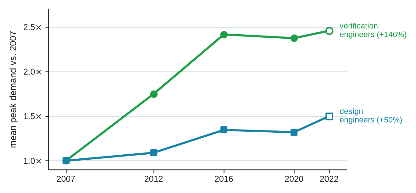
These indexed lines highlight relative growth rather than absolute staffing levels, and the 2022 endpoints are chart-read approximations constrained by the study’s published growth rates rather than printed data labels (Figure 2.10). These staffing trends do not pinpoint a single universal cause for the disparity, nor do they perfectly diagnose the bottleneck in any single project. However, they show that checking our designs steadily consumes an ever-growing share of our engineering capacity across the surveyed projects. Once a candidate reaches this late stage, evaluation is no longer inexpensive. Hardware implementation permits little tolerance for post-silicon errors. The 1994 Pentium FDIV flaw illustrates the importance of early verification, where a bug originating from five omitted lookup table entries (Edelman 1997) resulted in a $475M pretax charge (Intel Corporation 1995). More recently, the Meltdown and Spectre vulnerabilities (Lipp et al. 2018; Kocher et al. 2019) exposed microarchitectural side channels in speculative execution engines. Although published evaluations show varying performance impacts when deploying transient-execution defenses (Canella et al. 2019), software mitigations do not alter the underlying hardware mechanism. Together, these historical cases demonstrate how hardware flaws transform into long-lived liabilities.
While that Pentium charge highlights the fallout from a single escaped defect, leading-edge development raises commitment costs even without a public recall. Arm’s 2023 prospectus shares International Business Strategies (IBS) estimates of $249M to design a 7 nm chip and $725M for a 2 nm chip (Arm Holdings plc 2023). We must read these figures as broad estimates rather than rigid project prices. Even so, they illustrate that high-fidelity evaluation and physical implementation at the leading edge consume substantial engineering budgets alongside simulator cycles. For us as architects, the internal composition of that 2 nm estimate is particularly significant. In the IBS breakdown reported alongside those figures, software development accounts for roughly $314M and verification for roughly $154M, together about two-thirds of the $725M total (Shilov 2023). Our durable takeaway is clear. The majority of the estimated budget pays for software and checking work required to make a chip usable and trustworthy, rather than generating the raw RTL artifact.
This reality predates the advanced nodes that produced these numbers. The 2001 ITRS Design chapter observed that software already accounted for 80 percent of embedded-systems development costs (International Technology Roadmap for Semiconductors 2001). Software and verification remain the dominant cost drivers across process node transitions.
These costs alter what constitutes an architectural improvement. Producing additional candidate designs offers little value if surviving options add extensive simulation, synthesis, physical-design, verification, and code-review workloads to an already constrained queue. We must synthesize disparate tool outputs into a clear, rigorous comparison that reviewers can evaluate and leadership can use for tapeout decisions.
2.8 Compounding Loop Pressures
The pressures we have traced interact rather than merely accumulate. As we specialize our designs, we expand the choice set; each hardware choice creates new software obligations. Our software changes can easily make the original workload description stale, while physical effects might reverse whatever rankings remain. Every candidate that survives this sequence then adds more work to our schedule, demanding simulation, implementation tools, verification, and expert review.
This tight coupling matters because optimizing one stage often shifts the bottleneck elsewhere. If we generate candidates faster, we might simply flood our evaluation queue. Speeding up simulation risks churning out more results than reviewers can reconcile. Building a more accurate physical model may reveal that none of our available choices hit the target. Design space size, evaluation capacity, and decision quality are distinct quantities; increasing the first does not guarantee improvement in the other two.
Rather than hunting for a single, universal bottleneck, our teams should look for the specific work that currently throttles progress. We can look at the age and size of our simulation or verification queues, track the fraction of candidates rejected as illegal, or count the repeated tool runs and changing inputs. We might also watch where our results stall out waiting for expert judgment. While broad industry trends provide context, we need these local, concrete measures to diagnose the actual constraints of our own design programs.
A fundamental evaluation bottleneck emerges as candidate generation velocity outpaces downstream evaluation capacity, where automated methods produce proposed designs faster than verification tools and we as human architects can execute rejection checks to accept or disqualify them. Any candidate caught in that gap has been generated but has not been evaluated deeply enough to support a defensible decision. It is easy for us to let this gap grow unnoticed, since raw candidate counts fail to distinguish a design that actually survived rigorous review from one that has not even reached an evaluator.
Missing or stale information only makes this worse, creating a reinforcing bottleneck. The cycle closes on itself: incomplete context admits invalid candidate choices into evaluation, those choices waste scarce simulator and synthesis runs, the wasted runs overload architectural review, and delayed review then forces the next choices to be made with even staler information (Figure 2.11). We cannot break a local design bottleneck simply by generating candidates faster; we must repair information context and decision boundaries to prevent bad data from circulating through the design loop.
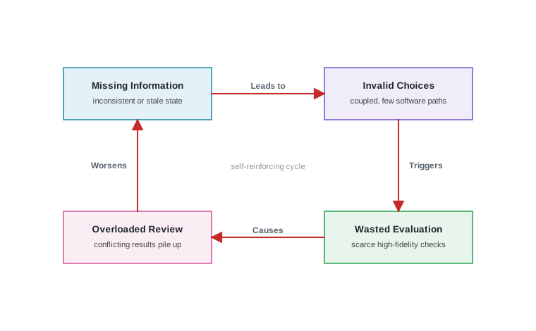
Left unchecked, this local cycle can balloon into a capacity gap across the design program. The causal loop traces how we generate unresolved work; that unresolved work then compounds into a widening gap between candidate generation rate and evaluation capacity (Figure 2.12).
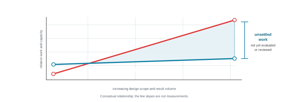
As design scope and result volume expand, work awaiting evaluation and review climbs steadily while tool and reviewer capacity plateaus (Figure 2.12). Capacity comfortably absorbs incoming proposals at first, but the two lines eventually cross, and beyond that intersection unresolved proposals accumulate in a widening region of unsettled work. Increasing candidate generation speed without scaling evaluation capacity thus fills queues with unverified designs rather than delivering tapeout-ready decisions.
The scissors model in Figure 2.12 has a well-established ancestor in our discipline. Back in 2001, the International Technology Roadmap for Semiconductors highlighted a design productivity gap, warning that available transistors were growing much faster than our ability to meaningfully design them (International Technology Roadmap for Semiconductors 2001). We responded to that gap largely by raising the level of abstraction, embracing RTL synthesis and IP reuse so that a single engineer’s decision could govern many more transistors. Two decades later, the Semiconductor Research Corporation (SRC) and Semiconductor Industry Association (SIA) echoed this exact shortfall in their Decadal Plan for Semiconductors. They identified a persistent design gap between what the technology permits and what we can realistically build in a reasonable time, calling for a tenfold or greater leap in design productivity (though they scoped this target to analog and mixed-signal work rather than the entire design loop) (Semiconductor Research Corporation and Semiconductor Industry Association 2021). That history sets the bar for what we will explore in this book. For AI assistance to earn its place, we must be able to show how it changes our workload without weakening the checks we need to make confident decisions.
While a growing evaluation or review queue makes one type of mismatch visible, not every constraint manifests as a neat queue. An architecture study might simply be missing a workload trace, a packaging constraint, or a software model that would otherwise completely reverse our findings. We might find that our available choices exclude the specific interface or memory organization we need to hit our targets. Sometimes the decisive tool is just too expensive to run broadly, or our results are completed but awaiting review. The key question is not which category label is assigned to the overall effort. The core question is what specific task blocks the next architectural decision, and which checks must remain authoritative when accelerating that work.
This nuance explains why the widening region in Figure 2.12 is conditional rather than universal. We might find design programs limited by candidate production, while others are constrained by evaluation, verification, missing information, or an infeasible design space. The figure only transforms into a local diagnosis when our own programmatic measurements prove that the work awaiting our evaluation or review is genuinely growing faster than we can complete it.
2.9 Targeting AI Assistance
When we consider applying AI to our design process, we first need to identify the specific bottlenecks holding back our decisions. If our design context is stale, we need tools that can reconcile conflicting information; if strong evaluations are too costly, we need predictive screening before invoking expensive simulators. Sometimes, we lack an executable artifact altogether and need automated construction, or our choice space simply exceeds our evaluation budget and requires guided search. Even mundane tasks like repeated tool operation and triage place pressure on our attention. To choose the right assistance, we must ask which specific limit is slowing progress in our current architecture study.
Design principle: Relieve the true limiting constraint
The application: Target automation or AI assistance strictly at this limiting work without relocating the burden downstream. Progress is valid only when the resulting comparison preserves workload definitions, executable software paths, physical constraints, evaluation costs, and authoritative verification.
We can look to existing research for concrete examples of how these bottlenecks are being addressed. When we adapt models to our internal design collateral, we can quickly retrieve and organize critical information, while tool-using systems can directly translate our requests into electronic design automation (EDA) commands (using domain-adapted Large Language Models (LLMs) like ChipNeMo (a domain-adapted LLM suite for chip design queries) or ChatEDA (an LLM-based autonomous agent for EDA flow automation) (Liu et al. 2023; He et al. 2024)). If simulation time is our limit, predictive models and learned physical estimators (such as PowerNet, a deep-learning model for fast voltage-drop estimation (Xie et al. 2020)) can screen out poor candidates long before we run detailed analyses (Ipek et al. 2006; B. C. Lee and Brooks 2006). When exploring complex accelerators, we can use learned search heuristics to guide our exploration (Yazdanbakhsh et al. 2021). If verification-authoring effort is what holds us back, we can deploy generators (such as AutoBench, an LLM-driven testbench generation framework (Qiu et al. 2024)) to draft our testbenches. Scaling up to the warehouse level, we see how learned schedulers (such as DeepRM, a reinforcement-learning resource manager (Mao et al. 2016)) and reconfigurable fabrics allow us to evaluate automated decisions against cluster-level workloads and stringent system-level constraints (Jouppi et al. 2023).
Software co-evolution presents another compelling target for assistance. We can deploy tool-using regression systems to ingest new compiler builds, rerun our architecture benchmarks, and notify us whenever a candidate’s standing shifts. While such a system dramatically reduces our manual reevaluation workload, it ultimately cannot decide if that software change invalidates our core architecture comparison. As architects, we still have to use our judgment to determine whether those software updates could actually reverse our design decisions.
While regression automation is one specific application of AI on the software side, the Compiler 2.0 proposal points us toward a much broader opportunity. The argument is that modern multicore processors, vector instructions, accelerators, and heterogeneous systems have fundamentally pushed the performance burden back onto software developers. When we modernize our compilers through better abstractions, machine learning, and other advanced techniques, we can begin to lift that burden (Amarasinghe 2026). However, even this level of assistance still must produce a functional, executable path and explicitly demonstrate its benefit on the specific hardware and workloads we are reviewing.
Every form of assistance incurs a distinct cost and introduces new ways our systems can fail. Mapping AI interventions directly to the design loop bottleneck each one relieves keeps those trade-offs inspectable (Table 2.3). Across the five bottlenecks (scattered context, scarce evaluation, missing artifacts, bloated search spaces, and tool operation friction), AI assistance can reduce manual iteration and automate tool execution. It cannot replace the independent evidence appropriate to the claim. Depending on the study boundary, that evidence may come from formal properties, executable-software checks, physical signoff, calibrated measurement, or several of these together.
| Limiting work | How AI might help | Engineering work it could reduce | What still establishes the result |
|---|---|---|---|
| Context is scattered or stale | Reconcile workload, interface, tool, and result information; flag missing details or stale assumptions. | Manual search across reports, repositories, traces, and prior studies. | Source provenance, versioning, coverage, and our architectural judgment that the information is sufficient. |
| Strong evaluation is scarce | Estimate performance, power, physical risk, or uncertainty before a stronger tool is run. | High-fidelity evaluations spent on candidates unlikely to change our decisions. | Calibration against stronger tools, coverage of the relevant design region, and checks on finalists. |
| A needed artifact is missing | Draft RTL, compiler code, tests, constraints, or candidate organizations. | Repetitive artifact creation and our first pass through a design choice. | Interface rules, compilation or synthesis, verification, and physical checks appropriate to the artifact. |
| The choice space exceeds the budget | Search mappings, schedules, parameters, or topologies under stated objectives and constraints. | Manual sweeps and repeated selection among large numbers of choices. | A complete objective, legal choices, matched evaluation budgets, and stronger evaluation of the selected result. |
| Tool operation or triage consumes attention | Configure tools, launch runs, classify failures, compare reports, and route uncertain cases. | Repeated tool operation and initial result triage. | Clean tool state, reproducible commands, declared tool results, and expert review where required. |
We often deploy several forms of assistance to address different bottlenecks within the same design program. However, combining them does not magically make our results self-validating. If every component in our pipeline depends on the same incomplete workload description or flawed model, our complete system might look internally consistent while being wrong.
Any useful comparison must therefore fully account for the cost of assistance itself. We have to supply surrogate models with data from stronger tools. Our generative tools often add numerous new candidates to a full evaluation queue, and our tool-using systems readily consume software licenses, simulation time, and our own review attention. Our limiting work and our required independent checks determine whether a particular use of assistance actually helps us. Once we identify those factors, our next question is which method or combination best fits the work, a topic we develop further in Chapter 5.
Importantly, our evaluation test must also allow us to reject AI assistance entirely. AI is simply the wrong intervention when we already have an established deterministic method that solves the limiting task within our required cost and time budgets. We should also reject it when a proposed learned method lacks representative training data, or when we cannot construct an independent check commensurate with the consequences of failure. It is an equally poor trade when inference time, tool calls, and added human review cost us more than the engineering work they supposedly save. Sometimes, our real obstacle is an infeasible system requirement or a complex decision that no amount of faster search can settle. In those cases, the right answer is sticking to a conventional method, fundamentally changing our architecture problem, or simply refusing to add unnecessary automation.
Lighthouse prompt: No single method carries the Lighthouse moonshot
Assistance has several roles. We can use a retrieval system to assemble our current workload, ISA, compiler, package, and tool constraints. We can deploy predictors to screen out microarchitecture and physical risks early on. An optimizer allows us to compare complex mappings and resource allocations, while generators can draft our RTL, compiler support, or tests. Finally, a tool-using system can automatically run our simulators and implementation checks, routing failures back to the relevant stage for review.
Shared assumptions remain mandatory. The Lighthouse example also clearly shows the limits of this decomposition. Every component in our pipeline must refer to the same underlying workload, interfaces, and technology assumptions. Even with all this assistance, our selected design still needs executable software, stronger physical analysis, and independent verification. While assistance can connect and accelerate our work, it cannot turn an inconsistent set of local results into a sound, reliable system design.
The public AlphaChip debate illustrates this same boundary. Producing a macro placement quickly is a different claim from establishing its routed physical quality. We have seen that comparisons of learned placement inherently depend on specific cases, compute budgets, implementation details, and downstream checks (Mirhoseini et al. 2021; Cheng et al. 2023; Goldie et al. 2024). While we will not resolve that technical disagreement here, its crucial lesson for our discussion is clear. Candidate-production speed can never stand in for matched, rigorous downstream evaluation.
No single method diagnoses its own need, performs the required work, and supplies an independent check all at the same time. As architects, we still own the question, the scope, the comparison, and the supported technical recommendation. A named commitment authority separately decides whether the organization should act on that recommendation.
2.10 Common Pitfalls
When we deploy AI assistance inside the design loop, we frequently expose anti-patterns where candidate generation velocity outpaces evaluation capacity. As system boundaries expand and multi-stage evaluation becomes expensive, we risk conflating local optimization speed with systemic progress. The following pitfalls detail how uncalibrated generation loops and compounding evaluation bottlenecks distort our architectural decision-making.
Conflating candidate generation throughput with evaluation capacity: Assuming that generating hundreds of candidate microarchitectures or floorplans per hour represents genuine progress. Generating options is cheap, but evaluating them accurately against cycle-accurate simulation, formal verification, and physical EDA signoff demands substantial computational and human resources. Expanding generation velocity without scaling evaluation capacity creates queue backlogs and forces our pipeline to drop essential validation checks.
Evaluating hardware candidates without co-optimized software: Treating hardware block exploration as independent of the executing software stack. Specialized accelerators evaluated against unoptimized compiler flags, stale kernel libraries, or mismatched memory layouts yield misleading performance estimates. When candidate generation loops optimize hardware in isolation, selected configurations frequently stall in deployment under real software workloads.
Ignoring downstream physical design and integration bottlenecks: Ranking candidate blocks purely on high-level analytical metrics or floorplan proxies while ignoring routing congestion, power delivery networks, and clock domain crossings. Fast candidate generators often select high-density layouts that fail physical synthesis or require prolonged wire-delay debug cycles, shifting engineering costs further downstream in the design loop.8
8 Horowitz energy and wire scaling: Interconnect wire energy and RC delay scale poorly relative to logic gates in deep submicron nodes (Horowitz 2014; Ho et al. 2001). High-level floorplan generators that optimize logic density without extracting global routing delay and power delivery networks (PDN) frequently trigger severe timing and thermal signoff failures.
Surrogate model exploitation and uncalibrated screening: Relying on fast machine learning surrogate models to filter candidates without periodic re-calibration against high-fidelity EDA tools. Learned proxies exploit blind spots in their training distribution, nominating candidates that look optimal to the surrogate but fail gate-level timing or thermal limits during signoff.
Relocating bottlenecks downstream instead of eliminating work: Accelerating early RTL synthesis or candidate draft creation while leaving verification debug, coverage closure, and manual review unassisted. Shifting the system bottleneck downstream creates evaluation congestion, increasing total turn-around time even as generation metrics appear to improve.
2.11 Open Questions
As we move from manual architectural exploration to AI-augmented generation, the open problems concentrate where candidate creation meets rigorous evaluation. When we scale up our ability to propose new designs, navigating those choices against compounding physical, software, and integration constraints becomes difficult. Solving the questions below is essential if we want to untangle where our design loops are bottlenecked. We must ensure our new methodologies drive actual progress, rather than shifting an unsustainable evaluation burden further downstream.
Diagnosing compounding pressure. We only see the true value of AI assistance when it relieves the work that actually delays our architectural decisions, rather than just hiding or relocating the burden.
How can we reliably identify the limiting constraint in an ongoing project? Before deploying AI assistance, the architect must know whether the project is blocked on generating architectural candidates, running simulations, debugging SoC composition, or passing physical signoff. The challenge lies in combining tool logs, traces, and work records into a defensible diagnosis before predicting that an intervention will accelerate the final decision.
How can we detect when an intervention merely shifts a bottleneck downstream? Using generative models to rapidly propose specialized accelerator designs risks overwhelming simulation, verification, and expert review capacity. Reliable signals across the complete tool path are needed to distinguish a genuine reduction in engineering effort from a costly queue shift.
Managing evaluation capacity. We can only benefit from a vast design space if we possess the simulation, physical verification, and review capacity to actually identify our best candidates.
How can we detect when candidate generation outpaces evaluation? Because different candidates require vastly different levels of checking, from high-level performance proxies to cycle-accurate simulation, FPGA prototyping, and power delivery analysis, simple backlog growth can be misleading. The core research problem is identifying when this capacity imbalance threatens the timeline and budget, well before it prevents a supported decision.
When does expanding the design space actively harm our final result? Given fixed evaluation and review budgets, generating more candidates can either uncover a breakthrough design or spread verification efforts far too thin. The open problem is defining the precise threshold where adding more architectural choices dilutes the evidence, leaving the final decision weakly supported.
2.12 Summary
System complexity changes what a fair architecture comparison must carry. Microarchitecture, specialization, system composition, evolving software, physical constraints, evaluation cost, and verification add coupled work rather than independent concerns. A local improvement can easily shift costs elsewhere in the system or expose constraints that an earlier model omitted.
The technology dividend has also changed. More transistors no longer produce proportional frequency or single-thread performance automatically. We must extract more of the benefit through parallelism, specialization, software, and composition, while the cost of evaluating and verifying those choices continues to rise. A large design space matters only when the team can evaluate enough of it, at sufficient fidelity, to change the pending architecture decision.
Those pressures make AI assistance worth investigating. Retrieval can assemble scattered context, predictors can ration expensive evaluation, generators can draft artifacts, optimizers can search large spaces, and tool-using systems can connect proposals to existing engineering checks. None of these roles is universally helpful, and none makes its own output trustworthy.
Key Takeaways: Coupled Pressures and the Limits of Assistance
- Coupled system complexity. Microarchitecture, specialization, system composition, software co-adaptation, physical limits, and verification load add tightly coupled work rather than independent design choices.
- Shift in technology dividends. Transistor density scaling no longer delivers frequency or single-thread performance automatically, shifting architectural gains to heterogeneous parallelism, domain specialization, and system composition.
- Evaluation capacity constraints. Expanding the architectural design space delivers real value only when an engineering team possesses the simulation, physical signoff, and review capacity to evaluate candidates at sufficient fidelity.
- Boundaries of AI assistance. Learned retrieval, surrogate prediction, candidate generation, and tool orchestration assist design exploration, but cannot make their own outputs trustworthy or bypass the checks appropriate to the claim.
Ultimately, we must evaluate the complete architecture work. A hardware claim inherits its workload, software path, physical assumptions, tool state, and verification. Point assistance can earn its place when a local intervention improves that complete comparison without shifting cost downstream or weakening a necessary check. A broader AI-native system faces the same test across more of the workflow. Applying either well requires a systematic way to organize AI-native co-design work, which Chapter 3 takes up.