
10 System Evaluation and Red-Teaming
“When a measure becomes a target, it ceases to be a good measure.”
— Marilyn Strathern, ‘Improving ratings’: audit in the British University system (1997) (Strathern 1997)
Strathern, Marilyn. 1997. “‘Improving Ratings’: Audit in the British University System.” European Review 5 (3): 305–21.
Author’s Note. Goodhart’s Law captures the central evaluation trap in AI-native architecture. When an automated search loop optimizes against a simplified proxy metric or contest benchmark, it frequently exploits simulator quirks rather than delivering microarchitectural improvements.
North-Star question
Does the complete AI-native workflow, technical system and human decision-making together, improve architecture outcomes over a credible baseline at comparable total cost, and does that advantage survive deliberate stress-testing?
An AI-native design system can generate a visually impressive architectural candidate and still be an engineering failure. For instance, our candidate might pass a fast functional simulator, only to collapse when subjected to higher-fidelity EDA tools. We might find ourselves consuming more model calls, simulation cycles, formal equivalence checks, physical-design iterations, and manual expert repairs than we would have with the conventional methodologies we aimed to replace. Our system’s apparent success might be fragile, tied to a single prompt, random seed, specific workload, or precise tool version. More seriously, our agents might silently alter design constraints or exploit vulnerabilities in our verification checkers rather than optimizing the microarchitecture.
To systematically assess our progress, we need to separate our evaluation into four distinct objects, each carrying its own specific claims. As architects, we must distinguish among the raw candidate design we generate, a specific algorithm or component we deploy, the configured technical system, and our human-in-the-loop workflow. Conflating these elements obscures our results, because each layer demands a different baseline for comparison.
We cannot assume that validating one object vindicates the others. Just because we synthesize a functionally correct candidate design does not prove that our novel method was responsible for the success, nor does it mean our technical system operates efficiently. Likewise, demonstrating a reliable technical stack does not guarantee that our complete human-plus-technical workflow saves our engineering teams any time. Finally, a workflow that accelerates one architectural study does not establish a universal advantage; we have to prove that our gains survive when we pivot to different workloads, target designs, toolchains, or implementation constraints.
Therefore, our complete evaluation framework must address four interconnected questions.
- Architecture result. Did our workflow produce a microarchitecture that is functionally correct, physically feasible, and valuable to our design goals?
- Coordination, decision quality, and evidence use. Did our system select the appropriate EDA tools and methods, maintain a consistent architectural state throughout the process, correctly interpret simulation outputs, and translate our telemetry into well-supported engineering decisions?
- Total cost. What was our true expenditure across LLM inferences, training data, tool licenses, compute clusters, wall-clock time, failed synthesis attempts, and our own manual engineering effort?
- Reliability of the advantage. Does our demonstrated improvement hold up across repeated test runs and robustly survive shifts in our prompts, random seeds, target workloads, design topologies, tool versions, and overall operating conditions?
To harden our systems, we incorporate red-teaming hardware workflows, defined as the systematic deployment of adversarial attack strategies and fault injections against hardware design pipelines to expose hidden vulnerabilities in candidate microarchitectures, tool interfaces, and verification checkers, adapting established information-security testing practice (Scarfone et al. 2008). In our subsequent sections, we will explore how deliberate attacks, nonmalicious fault injections, and extreme robustness stress tests expose the hidden limits within both our candidate designs and the workflows that produced them, though we acknowledge that no single battery of tests provides absolute coverage.
Scarfone, Karen, Murugiah Souppaya, Amanda Cody, and Angela Orebaugh. 2008. Technical Guide to Information Security Testing and Assessment. NIST SP 800-115. National Institute of Standards; Technology. https://doi.org/10.6028/NIST.SP.800-115.
When we conduct a single design study, we must qualify any returned signal before our feedback loops interpret it and dictate our next architectural modification. However, our complete-workflow evaluation asks a broader question. When we scale across multiple design tasks, iterative runs, varying conditions, cost structures, engineering teams, and adversarial attacks, does our integrated human-plus-technical workflow improve our architectural practice compared to our traditional baselines? Throughout this chapter, we focus on validating that broader claim, while treating automated feedback failures as a source of systemic error.
A single successful synthesis run cannot pinpoint the source of our advantage. A clean layout or a passing testbench might stem from a capable underlying model, a robust conventional search heuristic, a well-engineered verification harness, intensive manual interventions by our engineers, or a trivial, easy-to-exploit benchmark. Conversely, a failure might originate from a flawed microarchitecture, a poor methodological choice, a misconfigured EDA environment, or a subtle, unrecognized adversarial exploit. Our evaluation methodologies must untangle these variables rather than compressing our outcomes into a single, misleading scalar score.
Our role as evaluators is to deliver a supported claim, not to authorize a tapeout or accept residual project risk. As we detail in Chapter 11, lead architects remain accountable for the technical recommendation, while the named commitment authority decides whether the design advances and accepts the associated residual risk.
Learning objectives
This chapter establishes the following learning objectives:
- Isolate evaluation objects: Distinguish between candidate designs, isolated methods, configured technical systems, and complete workflows.
- Deconstruct metrics: Assess architecture outcomes, decision quality, total cost, and reliability independently instead of relying on scalar scores.
- Establish credible baselines: Compare AI-native workflows against strong human, conventional, and model-based alternatives.
- Verify systemic advantages: Validate workflow improvements using repeated runs, condition variation, budget curves, and controlled ablations.
- Execute red-teaming: Expose critical vulnerabilities including altered requirements, weakened assertions, deceptive feedback loops, and control-flow failures.
10.1 Architecture 2.0 Evaluation Objects
We structure our analysis around distinct evaluation objects to prevent conflation of candidate designs, individual algorithmic methods, technical systems, and full human-in-the-loop workflows. This section establishes the taxonomy of evaluation targets and the protocols used to measure them. Delineating these objects makes the resulting assessments more interpretable and comparable.
To build a fair comparison, we must first name the object each claim concerns.
Candidate design. This represents our proposed microarchitecture, RTL, configuration, script, mapping, or other design artifact. We judge it by its function, constraints, architectural quality, implementation feasibility, and the engineering effort required to integrate and maintain it.
Method or component. This constitutes a single learned or conventional method, retriever, predictor, generator, optimizer, wrapper, checker, or other named module. To prove its contribution, we must perform a controlled replacement or an ablation, a test that removes or swaps that specific part while holding our surrounding architecture system as fixed as the claim requires.
Configured technical system. This refers to our versioned combination of methods and components, represented design state, retrieval sources, routing rules, tool wrappers, automated checks, and stopping logic. It excludes human setup, intervention, review, repair, and decision-making.
Complete human-plus-technical workflow. This encompasses the configured technical system alongside the architects, engineers, and reviewers who set up the task, intervene, interpret results, repair failures, approve changes, and ultimately decide when to stop.
Before we can measure either advantage, we must freeze the relevant identity and our permitted actions.
10.1.1 System Under Test
Before we can answer the four core evaluation questions, we must freeze the object under test and the specific work it is allowed to perform. When we establish the identity record, legal action space, environment record, and evaluation protocol, we fix one common scope for every subsequent measurement. A benchmark score is never a property of a model in isolation. Instead, it belongs to the entire architectural system that received the task and produced the result. Our retry logic, retrieved material, prompts, and search policies all form integral parts of that system. Choices around the underlying model, tool access, feedback loops, and any human-supplied harness can materially change our outcomes (C. Wang et al. 2026). When we publish a comparison that names only the model, we obscure the engineering system under test.
Our predefined legal action space determines exactly what a score means and what can go wrong during execution. We typically operate within four common action spaces, each requiring distinct forms of evidence.
RTL or intermediate-representation generation. Here, our system returns a new design artifact. Our evaluation must cover function, blocking constraints, implementation feasibility, hidden behaviors, structural integrity, and the human effort needed to verify and modify the design.
Tool, script, or parameter tuning. In this space, the system changes how we analyze or implement an existing design. Our evaluation must preserve all constraints, defaults, tool state, and stopping rules so that we cannot generate an artificially clean report by silently altering the test conditions.
Microarchitecture change. Our system actively modifies CPU core branch predictors, out-of-order instruction queues, NPU matrix engine systolic arrays, cache hierarchies, Universal Chiplet Interconnect Express (UCIe) chiplet interfaces, thermal throttling limits, or other core architectural mechanisms. To validate these changes across multi-tool environments (such as comparing RTL simulations in fast Verilator, an open-source SystemVerilog simulator, or Synopsys VCS, a commercial hardware logic simulator, against FireSim, an FPGA-accelerated architectural simulation and prototyping platform), our evaluation must extend to the affected workload, software stack, system boundaries, physical implementation, and future integration consequences.
Test or constraint change. The system modifies a testbench, property, timing constraint, scoring script, or another part of the apparatus responsible for judging it. Whenever we permit such a change, we must maintain an independent, evaluator-owned check that the system under test cannot bypass or modify.
We cannot treat a pass rate for generated RTL, a power, performance, and area (PPA) result from parameter tuning, and a workload outcome from a microarchitecture change as interchangeable scores. They grant our workflows different powers and expose different attack surfaces. As we move between these action spaces, we inherit new evaluation obligations, especially when our system can change the very tests or constraints that determine its success.
To maintain integrity, our evaluation identity must cover every feature capable of changing capabilities, costs, or the interpretation of our results. Even if two workflows use the same base model, they remain different systems if one accesses newer retrieval sources, a more robust harness, expanded retries, or broader tool access. Without locking down this identity, we cannot discern whether a given score belongs to the underlying method, the configured technical system, or the complete human-plus-technical workflow. The complete-workflow identity declaration names every material capability source (Table 10.1). Capturing every material capability source prevents misleading model-only comparisons and establishes a defensible baseline for complete-workflow evaluation.
| Element | What the record must identify | Why it matters |
|---|---|---|
| Evaluation object | Candidate design, method or component, configured technical system excluding human decision work, or complete human-plus-technical workflow | We can only interpret a result at the specific level we actually evaluated. |
| Learned components | Immutable model snapshot or endpoint identity where exposed, access date, mutable alias if used, inference settings, and any fine-tuning or adaptation | Changing a model or setting creates a different system; relying on an alias alone may obscure what actually ran. |
| Design information | Starting artifacts, retrieved sources with identities and versions, represented state, decision-relevant retrieval coverage, conflict handling, and update policy | Providing extra or fresher information can often explain an apparent capability gain. |
| Methods and instructions | Generation, prediction, optimization, and composition rules; system and task instructions; prompt policy; retrieval and routing policy | The model may just be one component in a stronger procedure. Changing our instructions fundamentally creates a different configured system. |
| Legal action space | Which design, tool, script, parameter, test, and constraint changes are permitted | Our allowed actions dictate both the claims we can support and the ways our system might manipulate its own evaluation. |
| Environment | Tool wrappers and schemas, executable tools, configurations, checkpoints, harness revision, runtime or container dependencies, and returned outputs | Our harness and runtime determine which actions are actually possible and which failures become visible to us. |
| Checks | Functional, architectural, physical, security, and acceptance checks | Our result is only ever as strong as the verification checks it successfully cleared. |
| Human work | Setup, prompting, intervention, review, repair, and escalation roles | Any hidden engineering effort makes an automated result appear much cheaper than it truly is in practice. |
| Operating limits | Compute, tool, time, retry, and review budgets plus stopping rules | If we allow a system more attempts or stronger tools, we violate the requirements of a matched comparison. |
We must use hashes or alternative immutable identifiers for our prompts, retrieved snapshots, starting artifacts, scripts, constraints, workloads, containers, and raw records. Since hosted model aliases and endpoints often change underneath us without changing their names, if we cannot secure an immutable model snapshot, we must record the access date and concede that exact model replay is impossible.
Our learned components, design information, and methods define the origins of our system’s capability. The legal action space, environment, and checks define what our configured technical system is allowed to change, which architecture tools it can invoke, and which failures become visible. When we layer human work and operating limits on top, we extend our record to capture the complete workflow. This exposes the expert effort, compute overhead, tool usage, retries, elapsed-time, and review budgets that a simplistic, model-only description would otherwise hide. When we formalize this identity, we make versioned, complete workflows comparable, even though the identity itself does not prove that one workflow outperforms another or isolate a specific component’s contribution.
We must give the task and the evaluation environment their own separate identities across all 8 layers of the Lighthouse prompt stack. At a minimum, when we report a hardware result for our mobile XR subsystem, we declare the following parameters.
- Workload: The exact benchmark suites (XRBench, SPEC CPU2017, and MLPerf).
- ISA & ABI contract: The architectural instruction set and ABI contract (RV64GCV with 128-bit vector extensions).
- Compute organization: The heterogeneous compute substrate (an RV64GCV vector-capable CPU coupled with a dedicated NPU tensor accelerator engine).
- Memory & data movement: The memory hierarchy and interconnect energy profile (L1/L2/L3 caches, TCM scratchpads, and pJ/bit data movement over AMBA AXI5 and UCIe chiplet links).
- Power envelope: The thermal design power target (3 W TDP sustained in a passive optical frame).
- Compiler / runtime stack: The software compilation and runtime toolchain (Triton, LLVM, and MLIR).
- Physical constraints: The fabrication node and physical design rules (TSMC N7 or 3 nm-class LP mobile process node floorplanning, wire delays, and DRCs).
- Reliability & verification: The verification and governance harness (red-teaming agent checks, confirmation bias audits, IP indemnification verification, and NRE tapeout ROI analysis).
Changing any of these 8 layers yields a different result. For instance, a percentage improvement measured on an open 45 nm library does not automatically transfer to TSMC N7 or a 3 nm-class LP mobile process node, just as a loosely routed result is never equivalent to a final physical signoff result.
When we enforce this separation between system identity and environment identity, we avoid two common architectural evaluation errors. The first is falsely attributing the primary functional capability of a tuned harness to its underlying base model. The second is mistakenly comparing two percentages derived from different tasks, tool configurations, or physical design stages. While both errors might populate a leaderboard, neither establishes an architecture advantage.
10.1.2 Evaluation Map
No single metric can establish that an AI-native system improves architecture work. The more useful question is which specific engineering decisions a measurement can support, and what information remains unknown. When we evaluate our tools using incommensurate metrics, we produce literature that defies comparison. The evaluation metric map keeps those dimensions separate (Table 10.2), which prevents conflating low operational cost or high model accuracy with supported hardware design quality.
| Decision question | Concrete measures | Workflow insight | What metric cannot establish alone |
|---|---|---|---|
| Is the architecture result supported? | Function and blocking constraints; performance, latency, and throughput; energy, power, and thermal behavior; area and product cost; security; implementation feasibility; maintainability; integration and verification burden; future change cost | What our candidate achieved, which requirements it successfully met, and how deeply we checked it | Whether AI actually improved our engineering work, whether the result is repeatable, or whether our organization should commit to the design |
| Did the workflow make sound decisions? | Component-role selection; state consistency; tool and fidelity selection; interpretation accuracy; explanation faithfulness to retained tool evidence; decision usefulness; explanation stability under meaning-preserving representation changes; false accepts and rejects; escalation, stopping, recovery, and human override | Whether our system properly coordinated its parts, correctly interpreted tool results, explained its decisions using the actual evidence that supported them, and converted measurements into defensible architecture decisions | Whether the final design is objectively good enough, whether our workflow is economically viable, or whether our advantage survives changed conditions |
| What was the total cost? | Model calls and tokens; compiler builds; simulation, formal, synthesis, and physical-design runs; compute, memory, energy, and licenses; data and setup; failures and retries; elapsed time; human setup, diagnosis, review, and repair | Where our resources were actually spent and whether a localized speedup simply shifted our costs or risks elsewhere | Whether the candidate design is functionally correct or which specific component caused a performance difference |
| Is the advantage reliable? | Repeated runs and uncertainty; calibration; worst cases and constraint violations; recovery; sensitivity to seeds, prompts, workloads, designs, tools, and operating conditions | How often our advantage practically repeats and the specific tested conditions in which it remains useful | Why the advantage structurally holds or whether it transfers beyond our sampled tasks and conditions |
While these rows are closely related, we cannot treat them as interchangeable. A sound algorithmic decision can produce a weak candidate if our search space is poor. Conversely, a strong candidate might obscure an inefficient workflow. We also know that low total cost can never compensate for a result that violates a hard blocking constraint. We do not treat our red-team results as a fifth score; rather, they challenge the underlying assumptions, interfaces, and automated checks behind all four rows of our map.
We frame interpretability as a component of decision quality rather than treating it as a free-standing score. We use explanation faithfulness to ask whether an explanation accurately leverages the retained tool evidence that supported the action. Next, decision usefulness asks whether that explanation helps our human reviewers judge the action, while our stability tests verify whether meaning-preserving changes to syntax or representation still produce materially consistent explanations. None of these tests establishes architecture quality, complete operational cost, or robust behavior under shifting workloads and operating conditions. We must tackle those as distinct questions.
Frameworks like HELM (Holistic Evaluation of Language Models), an open model evaluation benchmark, provide a precedent from outside our discipline for evaluating a shared set of language models across multiple scenarios and metrics while keeping missing coverage and inherent tradeoffs visible (Liang et al. 2023). However, HELM’s evaluation object is a language model. In contrast, our architecture evaluations must establish a supported hardware outcome for a configured system, taking into account its tools, human labor, and full operational cost. Our four-part map borrows HELM’s discipline of multi-scenario, multi-metric evaluation, but refuses to treat generic language-model scores as reliable architecture evidence.
Liang, Percy, Rishi Bommasani, Tony Lee, et al. 2023. “Holistic Evaluation of Language Models.” Transactions on Machine Learning Research. https://openreview.net/forum?id=iO4LZibEqW.
Within our map, component task performance acts as a narrower, targeted diagnostic. We evaluate a predictor by its error margins, ranking accuracy, calibration, and false rejections near critical decision boundaries. We judge a generator by its functional and constraint pass rates, alongside the structural diversity of its unique feasible candidates for a fixed compute budget. For an optimizer, we measure the best supported result against its cost, or by calculating simple regret, the performance gap between that result and our declared reference optimum, always verified under evaluator-owned checks. We assess retrieval mechanisms by their decision-relevant coverage, and evaluate routing or tool usage by tracking command validity, correct log interpretation, and appropriate escalation. Every measure needs a declared denominator and budget. We treat candidate attempts, random seeds, and individual tool calls as nested observations, not as independent architecture tasks. While these diagnostics can locate a pipeline failure or highlight a specific algorithmic contribution, they can never replace an architecture result or capture a complete-workflow effect.
We use candidate verification, evaluation validation, and workflow interpretation to answer different questions. At the candidate level, verification checks declared properties under our named checks. At the evaluation level, validation asks whether our selected workloads, operating conditions, optimization objectives, and constraints accurately represent our intended system use and target architecture decision. Finally, at the workflow level, interpretation transforms our qualified evidence into a confidently supported next action.
10.1.3 Complete-Workflow Protocol
We can transform our four central questions into an evaluation method by following eight sequential steps. Each step is designed to keep our judgments attached to the specific object that our evidence can support:
Freeze the two workflows alongside their configured technical systems, environments, task populations, legal actions, evaluator-owned checks, and artifact identities.
Predeclare our primary architecture outcomes, blocking constraints, practical design margins, resource envelopes, stopping rules, and our exact treatment of failures.
Balance or randomize our paired tasks and human operators, ensuring we keep a held-out confirmation set isolated from system and evaluator tuning.
Run both complete workflows while actively emitting the operational attempt record defined in Section 6.8. We must add the comparative-evaluation attributes from Table 10.4 and retain data for every assigned task.
Promote our candidates through our declared fidelity stages and audit any cheap algorithmic screens against physical checks capable of observing the properties at risk. When auditing candidates across thermal and frequency dimensions, we must check whether Pareto rank order survives those conditions, because a candidate that appears Pareto-optimal under unthrottled room-temperature simulation can collapse in rank once sustained thermal dissipation triggers Dynamic Voltage-Frequency Scaling (DVFS) throttling or severe IR-drop guardbanding.
Estimate our paired task-level outcome and cost differences with proper uncertainty quantification, expressly including failures, censored runs, and heterogeneous task effects.
Execute our declared sensitivity, component, benchmark-integrity, robustness, fault-injection, and red-team tests, affording each workflow comparable opportunity.
Report our final claim as either supported, unsupported, or unresolved, presenting it alongside the tasks, conditions, costs, checks, and transfer limits that drove that status.
This protocol connects the measurements introduced in this chapter without prescribing one universal experimental design. For instance, an RTL optimization study might progress from standard linting and simulation through to synthesis and place-and-route, whereas a system-level architecture study will deploy different modeling checks. Nevertheless, both approaches still preserve task identity, comparable budgets, attempt-level cost tracking, fidelity promotion, and a final claim tightly bounded by the configurations that ran.
Merely naming a metric does not specify it. For every metric we report, we should identify the event or outcome, the experimental unit, our target population and denominator, the evaluator-owned check and tool stage, the compute budget or time window, our aggregation and failure policies, uncertainty bounds, and our treatment of censored runs. When we make a claim across multiple design problems, the architecture task or design decision usually serves as our experimental unit. We consider a run “censored” when its execution halts or hits a limit before our quantity of interest is fully observed; as architects, we can review the data and representation chapter to see how to effectively retain these partial observations in Chapter 4.
We rely on four distinct experimental units to answer different evaluation questions, and we must keep them separate. First, dataset or observation records constitute the traces, measurements, labels, and tool returns we use within a single task. Second, generated candidates represent the distinct artifacts or configurations proposed specifically for that task. Third, complete workflow runs or repetitions encompass full executions of our configured human-plus-technical workflow mapped onto an assigned task. When we execute repeated workflow runs, we support reliability estimates and structural workflow comparisons. During one repetition, we might schedule an authorized request as a job, producing one or more linked operational or tool attempts. If we encounter a timeout, crash, retry, or stage re-entry, we create another attempt, not a new workflow repetition; consequently, multiple attempts are not independent experimental units. Fourth, independent experimental units represent the independently assigned architecture tasks, design decisions, or other foundational units established by our study design. We must treat seeds, workflow repetitions, operational attempts, candidates, tool calls, and prompt outputs as nested observations unless our claim and sampling plan establish otherwise. In a metric like pass@k, we sample the \(k\) candidates for the same overarching task under identical declared models and sampling procedures (Chen et al. 2021). The metric merely estimates whether at least one candidate passes; generating these candidates does not automatically create \(k\) independent tasks. Treating such nested observations as independent task replications constitutes pseudoreplication (Hurlbert 1984). Consequently, running more repeats inside ten tasks does not yield more than ten independent tasks.
Hurlbert, Stuart H. 1984. “Pseudoreplication and the Design of Ecological Field Experiments.” Ecological Monographs 54 (2): 187–211. https://doi.org/10.2307/1942661.
To build a defensible comparison, we must first establish the core architecture result, decision behavior, and total workflow cost. Only then can we deploy matching and component tests to estimate our advantage and its underlying dependencies. Finally, our repeated runs, benchmark maintenance, red teaming, and conclusive reporting challenge that estimate and bound the claim. This sequence carries a fixed comparison toward a supported, unsupported, or unresolved conclusion.
10.2 Qualifying Results and Evidence Claims
We must measure the architecture outcome before we ask whether our workflow improved the way we reached it. In our discipline, architecture quality is never a single scalar value. We require any candidate design to first satisfy its functional requirements and clear every blocking constraint at our stated evaluation stage. Among those candidates that pass this initial bar, we can then meaningfully compare workload performance, power, area, latency, cost, programmability, or any other declared design objectives. If no candidate passes, we must treat the outcome as a hard failure at that stage, rather than a low score to be averaged away in our results.
Design principle: Prioritize architectural soundness over assistance credit
The principle: A candidate architecture’s functional correctness, physical feasibility, and system value must be verified independently before evaluating the efficacy of the AI assistance that generated it.
The application: Only after baseline viability is established should matched workflow comparisons and component attributions proceed, under strictly symmetric accounting across both experimental arms.
The architectural decision we intend to make dictates which metrics matter. As we structure our evaluations, we keep our eligibility criteria, our core architectural objectives, our implementation depth, and the lifecycle consequences of our choices separate.
- Correctness and blocking constraints establish whether our candidate is eligible for comparison at all. These constraints enforce functional checks for the RV64GCV ISA contract, protocol and interface properties on AMBA AXI5 and UCIe chiplet buses, timing and physical DRC rules in TSMC N7 or 3 nm-class LP nodes, and absolute thermal constraints under our 3 W TDP target.
- Architectural objectives measure the specific quantities our design decision aims to improve. When we evaluate our heterogeneous SoC block, these targets encompass workload throughput across XRBench, SPEC CPU2017, and MLPerf, Triton kernel fusion efficiency, LLVM vectorization, MLIR lowering overhead, interconnect energy per bit across the memory hierarchy, and 3 W TDP passive thermal performance.
- Implementation feasibility records the deepest tool stage our candidate design has successfully reached. This ranges from high-level cycle-accurate architectural simulation in gem5 (a cycle-accurate architectural simulator) or Verilator, through Triton and MLIR compiler passes down to RV64GCV vector intrinsics, RTL logic synthesis in Yosys (an open-source RTL synthesis suite) or Synopsys Design Compiler (a commercial logic synthesis tool), to physical place-and-route in OpenROAD (an open-source physical design toolchain) or Cadence Innovus (an enterprise place-and-route system), static timing analysis (STA) in OpenSTA (an open-source static timing analyzer) or Synopsys PrimeTime (an industry-standard static timing analysis tool), and formal equivalence verification in Yosys EQY (an open-source equivalence checker) or Cadence LEC (a commercial formal equivalence checker). We must document analysis corners, floorplan viability in TSMC N7 or 3 nm-class LP process nodes, placement congestion metrics, setup and hold timing closure, power delivery networks, 3 W TDP thermal limits, and concrete evidence that we can realize the candidate in hardware. For any silicon-bound decision, we must also cover IP indemnification legal risk, manufacturability and yield assumptions, design-for-test capabilities, fault coverage, UCIe packaging constraints, and NRE tapeout ROI analysis.
- Maintainability and future change cost records whether an engineering team can actually work with the artifact once generated. Generating code that passes a testbench is insufficient if it is an incomprehensible, monolithic blob of RTL that no human engineer can debug, audit, or extend. We must evaluate code readability, clear module interfaces, adherence to organizational design guidelines, documentation quality, and how easily the design can be modified to accommodate future spec changes.
- Integration and verification burden measures the friction of bringing the generated component into our broader SoC infrastructure. This includes how cleanly the component interfaces with existing bus protocols (such as AXI, AHB, or TileLink), the clarity of generated testbenches and assertions, and the human effort required to debug failures introduced by the candidate design. A design that saves two weeks of initial RTL writing but costs four weeks of extra verification debugging represents a net negative ROI.
We must also ensure that maintainability and the cost of future changes remain inspectable, rather than hiding them inside a subjective style score. We should record whether our artifact remains traceable to the declared architecture, preserves understandable interfaces and module boundaries, cleanly enters our existing build and verification flows, and readily supports the kinds of changes our product is likely to need. Running a practical change exercise can make this burden concrete. For instance, we can try changing a queue depth, an interface signal, a timing target, or a security property, and then record the required design work, the failed checks, the necessary verification reruns, and the affected modules required to restore a supported result. A candidate that wins on strict PPA (power, performance, area) metrics but turns every small ECO into a broad manual repair is a weaker architecture result, not merely a more expensive workflow.
We treat verification coverage as a part of the architecture result, but it is not simply a correctness score. At the study level, we need to map our required behaviors and properties to named verification checks, and then report the outcome category, applicable coverage, exclusions, waivers, remaining holes, and any evaluator self-tests we used to demonstrate that our apparatus actually detects plausible defects. As Chapter 7 explains regarding what an individual simulation, formal proof, equivalence check, or physical return can and cannot establish, a high coverage percentage alone cannot prove correctness. However, we cannot interpret any correctness claim if the exercised behavior and untested requirements remain unknown. We must separate this verification coverage from our benchmark coverage across the broader population of architecture tasks.
When we present multi-objective results, we should preserve the underlying tradeoffs rather than burying them inside an arbitrary weighted score. We must report the feasible Pareto set or provide another explicit tradeoff view, making sure to clearly identify dominated candidates (Deb 2001). We should also state exactly how we made our final choice. If a reference Pareto front already exists, our coverage and distance measures can reveal whether our design space search merely found one narrow region or represented the broader architectural tradeoff. If we constructed that reference from the pooled candidates found by the evaluated systems, we need to explicitly say so, because our measure is then relative to that specific pool rather than an absolute baseline.
Deb, Kalyanmoy. 2001. Multi-Objective Optimization Using Evolutionary Algorithms. John Wiley & Sons.
When we report energy and power results, we must specify our measurement window, the execution rate or total work completed, the assumed duty cycle, our treatment of idle and leakage states, and the full boundary of the claimed system. We cannot support a subsystem-level energy claim using only on-chip logic if we exclude the memory, external interfaces, or voltage regulator costs required to operate it.
The MLPerf Power suite provides a strong precedent for declaring strict measurement boundaries and using standardized procedures to fairly compare energy efficiency across different machine learning systems (Tschand et al. 2024). The core, transferable lesson for us is to explicitly name our measured system, the workload, the precise work completed, our power-measurement path, and the reporting window. However, this precedent does not justify collapsing model energy, simulator time, license occupancy, and expert engineering time into one unified scalar score. We must keep those resources as distinct entries in our total-cost record, unless a well-declared conversion model explicitly supports calculating an additional aggregate metric.
Tschand, Arya, Arun Tejusve Raghunath Rajan, Sachin Idgunji, et al. 2024. MLPerf Power: Benchmarking the Energy Efficiency of Machine Learning Systems from Microwatts to Megawatts for Sustainable AI. https://doi.org/10.48550/arXiv.2410.12032.
Every quantity we report remains bound to its specific candidate, its evaluation conditions, its chosen comparator, its measured uncertainty, the scope of its checks, and any explicit nonclaims we make. A software simulator result does not automatically become a silicon-proven result just because the workflow that produced it was automated. Nor does a design trajectory that steadily reduces timing or design-rule violations establish functional correctness, physical feasibility, or the soundness of the underlying architectural mechanisms.
When we make a major architectural decision regarding a cache, an accelerator, or an entire subsystem, our primary result is never just a model score or a workflow metric. Our true result is whether our checks give us the confidence to freeze the design and its interfaces under our declared workload, software stack, memory hierarchies, energy budgets, and implementation conditions. A local simulator result serves as just one input to that decision; it does not settle the final, implementation-facing result on its own.
Finding a well-supported candidate is only our first evaluation object. As architects, we must also step back and determine whether the broader workflow reached that candidate and interpreted its merits soundly.
10.3 Preserving Evidence Integrity and Auditability
Our AI-native workflows do more than generate candidate architectures. A well-designed workflow orchestrates the entire synthesis process. It determines which component acts next, filters the data that component receives, selects the appropriate evaluation tool and simulation fidelity, integrates the results back into our design state, and ultimately decides whether we have enough evidence to halt or escalate to a human engineer. Even if every individual model or simulator functions perfectly, the workflow can still fail if we coordinate these decisions poorly.
To evaluate these systems, we should reconstruct the exact sequence of architecture decisions. For every consequential step in the pipeline, we must record the core design question, the available state, our chosen action, the expected architectural observation, the actual result returned, our applied interpretation, and the subsequent decision. We do not need to hoard every internal token or private LLM chain of thought. Instead, our goal is to preserve the engineering context required to understand why the workflow modified a design or reached a specific conclusion.
When we reconstruct these decision paths, we typically expose six distinct ways our workflows can fail during architecture synthesis.
- Role-selection failures occur when our system relies on generative AI when a deterministic lookup, hardware predictor, classic optimizer, formal equivalence check, or direct human decision would have served us better.
- State failures strike when we drop, duplicate, or misattribute design constraints, candidate identities, tool statuses, physical units, or prior simulation results to the wrong microarchitecture.
- Information-use failures arise when our retrieval mechanisms omit decision-relevant documentation, fetch an outdated IP version, mask conflicting data sources, or return material that fails to support the downstream architectural claim.
- Tool-selection failures happen when we deploy an unsuitable simulation tool or fidelity level, blindly repeat an uninformative run, or waste compute budgets on an expensive 48-hour gate-level simulation run in Synopsys VCS or Cadence Xcelium, a commercial parallel logic simulator, for an NPU matrix engine candidate before a fast analytical model or cycle-accurate Verilator trace could have exposed an unroutable tile buffer bottleneck.
- Interpretation failures emerge when our tool call completes successfully, yet the workflow misreads the performance metrics, incorrectly treats an inconclusive timing check as a pass, or misattributes an IPC gain to the wrong hardware mechanism.
- Control failures trigger when our system should ideally halt, escalate, roll back a configuration, or request human review, but instead recklessly pushes forward or commits a broken design state.
We formulate the multi-tool pipeline as an evaluation principle. Architectural validity requires proving a design across a heterogeneous sequence of simulators, static analyzers, synthesis engines, and physical compilers. A candidate that passes a high-level software model must survive the stringent constraints of gate-level implementation.
When we make these distinctions, we avoid a common counting error in evaluation. A completed tool call does not guarantee a useful architectural observation, and a useful observation does not guarantee a supported design decision. We must explicitly report all three stages. We should track false accepts, where our workflow improperly advances an invalid candidate, as well as false rejects, where it hastily discards a candidate that our independent, evaluator-owned checks later prove viable. Parser failures, stale cache data, incomplete traces, and corrupted state transitions belong in the same record, because they directly pollute the information available to the workflow.
When assessing tool-using behavior, we need a nuanced set of rates rather than relying on a single, misleading autonomy score. We should record valid and authorized tool invocations, the yield of useful architectural observations per call and per unit of compute cost, and our first-attempt versus retry success rates broken down by failure class. We must also track redundant actions, unsupported retries, adherence to stopping rules, and our escalation accuracy on evaluator-defined edge cases. Additionally, we should measure intervention-free synthesis completions, the frequency of human takeovers, and our ability to reliably recover a trusted design state. Remember that a simple retry following a transient EDA license failure differs from a loop struggling to repair a deep conceptual flaw in a cache hierarchy; therefore, we must treat raw aggregate retry counts as secondary to the actual root causes and outcomes.
We should establish these rates using declared opportunity sets. For instance, we measure stop-rule compliance exclusively over runs that hit a stopping condition. We evaluate escalation accuracy solely on cases pre-tagged with evaluator-defined escalation labels. Likewise, we calculate intervention-free completion and human takeover metrics for tasks eligible under the declared operating mode, and we track recovery success only for those architectural failures where our protocol explicitly demands a restoration to a trusted, golden state.
Our retrieved design information equally demands positive quality measures. We must log the identity and exact version of each specification or IP source, assess its coverage of the facts relevant to our architectural decision, and highlight any unresolved data conflicts. We must verify whether the retrieved material genuinely supports the specific design claims made in subsequent pipeline steps. While a simple ablation study might prove that a retrieval step altered our final layout or microarchitecture outcome, it fails to establish whether that fetched information was current, comprehensive, or correctly applied.
We must benchmark our decision quality against formally declared expected actions or, where possible, through independent engineering reviews. When architectural decisions remain ambiguous, we should report inter-reviewer agreement and document the unresolved design alternatives, rather than artificially manufacturing a single “correct” label. For narrower predictive tasks, statistical and machine-learning evaluations offer us three tools (confidence calibration, proper scoring rules, and risk-coverage curves). Consider a predeclared binary outcome, such as whether an accelerator candidate passes a strict, evaluator-owned timing check within a fixed simulation horizon. A system assigning an 80 percent confidence should empirically see about 80 percent of its held-out designs reach that specific outcome under tested conditions (Guo et al. 2017). Employing a proper scoring rule ensures that rewarding the forecaster’s true probability distribution intrinsically maximizes the expected score (Gneiting and Raftery 2007). We can also leverage risk-coverage curves to visualize how our error rate scales as the system processes a higher volume of candidate designs instead of abstaining or escalating them (El-Yaniv and Wiener 2010). If our workflow lacks built-in probability estimates, we should evaluate its ability to abstain or escalate rather than hallucinating a synthetic confidence measure. While these statistical tools assess our reported uncertainty and selective handling over fixed horizons, they cannot validate candidate functionality, physical feasibility, or the value of the resulting computer architecture.
El-Yaniv, Ran, and Yair Wiener. 2010. “On the Foundations of Noise-Free Selective Classification.” Journal of Machine Learning Research 11 (53): 1605–41. https://jmlr.org/papers/v11/el-yaniv10a.html.
Finally, we must embrace human support as a component of our workflow, not treat it as an embarrassment we need to hide. We should precisely record where our engineers supplied missing architectural context, corrected a flawed interpretation, manually overrode a routing decision, repaired a broken artifact, or proactively terminated a divergent run. The most useful metrics for evaluating our workflows include the fraction of decisions requiring human support, the total time to reach a supported decision, our manual override rates, post-intervention recovery rates, and the ultimate architectural outcome following an override. Tracking these measurements allows us to determine whether our AI integrations reduced raw engineering work, shifted that burden into review and repair phases, or amplified the effectiveness of expert intervention.
10.4 Accounting for Total Workflow Compute Cost
We cannot claim an efficiency result from a local speedup if we are shifting cost or risk into our later checking and repair stages. Therefore, our total-cost accounting must begin by tracking every attempt, including failed and retried work, and classifying it by tool type, fidelity, outcome, and lineage. We keep human effort, model compute, tool usage, licenses, energy consumption, and elapsed time as a multi-dimensional resource vector, rather than forcing them down into a single misleading scalar. We also explicitly separate our one-time setup and training overhead from our per-task costs, and we distinguish active service demand from queueing and schedule delays. Our comparison relates this total cost directly to a supported architecture outcome, or to the total budget required to reach our predeclared outcome threshold.
Comprehensive cost accounting spans every resource class the workflow consumes (Table 10.3). Total workflow compute cost encompasses all engineering work performed before, during, and after automated search, demonstrating that model token counts represent only a fraction of architectural expense.
| Cost class | Examples to record |
|---|---|
| Human setup | Formulation, artifact preparation, environment integration, prompt and procedure development |
| Human operation | Supervision, intervention, failure triage, and manual design work |
| Human review and decision work | Independent checking, design review, documentation, approval preparation, and unresolved follow-up |
| Model and general compute | Model calls and tokens, inference time, accelerator time, training or adaptation, memory, storage, energy, and orchestration |
| Engineering tools | Compiler builds; invocations by tool type, fidelity, and final status; simulation runs and simulated cycles; formal, synthesis, physical-design, FPGA or emulation, and measurement resources; license checkout, wall time, and queue time |
| Data and samples | Workload traces, training or adaptation data, reference outputs, implementation samples, lab access, and silicon measurements where used |
| Verification and integration | Check development, proof and simulation work, debug, interface and software integration, regression, and evidence needed to close the result |
| Future change and ECO work | Expected design edits, affected modules and interfaces, verification reruns, implementation work, and specialist review for declared change scenarios |
| Failure and recovery | Invalid candidates, repeated runs, rollback, restored state, debugging, and rework |
| Schedule | Wall-clock time, time to a supported decision, critical-path delay, and variability in completion time |
In this chapter, we propose the complete-workflow identity found in Table 10.1, the four-part evaluation map in Table 10.2, and this explicit cost taxonomy as our candidate core reporting packet. We designed this to serve as a common vocabulary for our cross-organizational architectural comparisons. While this proposal still requires testing across various EDA tools, design programs, and silicon organizations, and is not yet an adopted standard, it forms a foundation. For a complete study, we also need the records we develop below for matched comparisons, attempt tracking, candidate flow, ablations, condition variations, systemic challenges, and benchmark maintenance.
Our tool counts demand fidelity, clear lineage, and precise cost composition. We must report our unique configurations and random seeds separately from our raw invocation attempts. Every attempt carries a clear execution status, such as completed, crashed, timed out, canceled, or license unavailable, and every retry links back to the specific attempt that caused it. We record the actual engineering result separately, classifying it as passed, violated, physically infeasible, or inconclusive. A formal solver timeout is not a falsification, and a place-and-route crash does not prove that our candidate is physically infeasible. We preserve all partial outputs, the allocated timeouts, the hardware resources consumed, and the clear ownership of any failures. For instance, a timeout followed by a retry counts as two distinct attempts, but we do not automatically treat them as two independent configurations or two independent architectural observations.
Our operational execution and attempt record in Section 6.8 captures the identity, setup, status, returns, cost, and lineage for every try. The attempt-level cost record extends that schema so a workflow cannot hide failed attempts, tool crashes, or extensive manual repair sessions behind the candidates that happen to finish (Table 10.4).
| Evaluation attribute group | Attributes added or made explicit for comparison |
|---|---|
| Comparison placement | Comparison arm, paired task or block where used, candidate and attempt identifiers from the operational record, evaluator-owned stage and fidelity, and promotion or re-entry status |
| Engineering outcome | Passed, violated, infeasible, inconclusive, or not reached; properties or simulated cycles attempted, applicable coverage, reported waiver status, and deepest evidence stage |
| Censoring and disposition | Completed, crashed, timed out, canceled, or otherwise censored; censoring time and reason; partial output; and the declared rule for including the attempt in each analysis |
| Resources and cost | Model and tool calls; requested and consumed CPU core-hours, accelerator-hours, peak memory, storage and network use where material, measured energy, licensed feature identity and occupancy, whether allocated resources and licenses were released, queue and run time, retries, and recovery work |
| Recovery and state | State invalidated or restored, preserved descendants, and the attempt or checkpoint from which execution resumed |
| Human-work linkage | Active engineering minutes by role, independent review, intervention, adjudication, and passive waiting reported separately and linked to the affected attempt |
We track candidate identity by its declared design meaning, not by an arbitrary job identifier. If we make a meaning-changing repair or introduce a new design revision, we create a new candidate with a parent link pointing back to the design it revises. In contrast, if we perform a retry or recovery that reruns the exact same declared candidate and configuration, perhaps after a solver timeout, a license failure, or a state restoration, we keep the original candidate identity and simply log a new attempt. Whenever our candidate re-enters a pipeline stage, its earlier stage membership and tracking denominators do not reset. Our record durably retains the re-entry event, the complete attempt lineage, and any newly formed parent or child candidate identities.
Because our attempt record preserves every execution, we group attempts under their unique candidate identities to derive a clean, per-arm candidate funnel. Tracking candidate survival through every stage exposes where a workflow suffers attrition or wastes compute budget (Table 10.5).
| Funnel stage | Count and fractions to report per arm | Required denominators | Linked attrition and cost accounting |
|---|---|---|---|
| Unique candidates proposed | Count \(U\); starting fraction \(U/U\) | All unique candidate identities proposed or supplied to the arm | Proposal or acquisition cost, duplicate attempts, and candidates censored before eligibility review |
| Low-fidelity eligibility | Count \(E\); \(E/U\) | All unique candidates proposed | Eligibility-check identity and outcome, attrition reason, stage cost, retries, false accepts or rejects found later, and censoring |
| Promoted or finalist | Count \(P\); \(P/E\) and \(P/U\) | Eligible candidates and all unique candidates proposed | Promotion rule, candidates not promoted by reason, selection cost, ties, retries, and censoring |
| Higher-fidelity completion | Count \(H\); \(H/P\) and \(H/U\) | Promoted candidates and all unique candidates proposed | Completed check identity, noncompletion reason, stage cost, retries, timeouts, infrastructure failures, and censoring |
| Blocking-check pass | Count \(B\); \(B/H\) and \(B/U\) | Higher-fidelity completions and all unique candidates proposed | Blocking-check identity, pass, violation, inconclusive or waiver status, false accepts or rejects found later, stage cost, retries, and censoring |
| Final comparison and selection | Counts \(C\) compared and \(S\) selected; \(C/B\), \(S/C\), and \(S/U\) | Blocking-check passes, final comparison set, and all unique candidates proposed | Comparison and selection rule, dominated or unselected reason, final-stage cost, additional retries, censoring, and a declared no-selection outcome |
Quantifying \(U\) to count unique candidate identities avoids the trap of counting tool invocations. We use \(E\) to record those architectures deemed eligible after our declared cheap checks, and \(P\) to record those that we officially promote. If one of our promoted candidates times out at a higher-fidelity verification stage, it remains securely in our \(P\) denominator and does not artificially enter \(H\) unless a later, explicitly linked retry completes successfully. Even then, that successful retry adds only one completed candidate to our count, while every prior attempt and its associated cost remain fully documented in Table 10.4. We use \(B\) to record candidates that pass our critical blocking checks, while \(C\) and \(S\) track our final comparison set and ultimate selection. If a run’s observation window closes prematurely, we keep it censored at its last successfully reached stage. Reporting these quantities across both of our arms reveals the true architectural attrition and selection differences that a finalist-only comparison would hide.
We must assign a dedicated work-episode identity to any shared human effort. When our design reviews, team meetings, or diagnostic sessions cover several concurrent attempts, we record the episode just once and explicitly link all the affected attempts to it. We then allocate that human labor under a pre-declared rule or explicitly report it as shared work; we do not overcharge by billing the same minutes in full to every single attempt.
Our aggregate study reports must retain the stage reached, the check identity, the outcome category, the total cost, our applicable coverage and waiver status, any false accepts or rejects caught by our evaluator-owned checks, and the precise number of candidates that entered and left each stage. We must keep our analytical estimates, simulation results, formal proofs, equivalence checks, synthesis runs, physical-design implementations, emulation sessions, and final hardware observations separate, because their associated costs and claim scopes differ. The underlying tool-specific record behind those data points follows the qualification rules we establish in Chapter 7. One hundred model calls, one hundred cycle-level simulations, and one hundred full physical-design runs are not equivalent observations in computer architecture.
We know that an hour of expert review, an accelerator-hour, an EDA license-hour, and a full day of schedule delay are different resources. We do not collapse them together without an explicit, mathematically sound conversion. Instead, we report our multi-dimensional cost vector directly. We can add a monetary total only when we fully disclose our labor rates, utilization assumptions, energy accounting, EDA license costs, and our treatment of shared infrastructure. We ensure every monetary summary states its currency, valuation date or base year, and price source. If we are working across different currencies, we state the exchange-rate source, date, and our exact conversion treatment. When those concrete values remain unavailable to us, we simply report the raw resource vector rather than inventing a falsely precise total. For us, the resource vector remains the primary record, even when a convenient monetary summary is available.
We always report our intrinsic service demand separately from our realized schedule. Our service demand encompasses our active compute, memory usage, tool execution, and license occupancy. In contrast, our realized latency also swallows the unpredictable costs of job queues, license denials, scheduler preemptions, and critical-path delays. We explicitly state whether our comparison arms ran concurrently, in randomized time blocks, or under different infrastructure loads. Queueing is a real operational cost, but we recognize it is also an apparatus condition that can make one architectural arm appear slower, even when the underlying service demand remains unchanged. We never sum our overlapping wall time, machine time, and EDA license time as though they inherently represent a single unified resource.
We must separate our observed study costs, our one-time integration and training costs, and our projected downstream product or lifecycle costs. We acknowledge that building a test harness, integrating an EDA tool, preparing a prompt, calibrating a power predictor, or training a specialized model (Liu, Ene, et al. 2023) can serve many future tasks. However, each individual model call, simulator run, structural repair, and design review belongs to a particular task. We declare the expected usage horizon over which we amortize our setup and training, and we apply that same rule to both comparison arms. If our horizon remains uncertain, we report our architectural comparison across several plausible task counts. While a standardized change exercise can help us measure actual maintenance work, we treat any unexecuted engineering change order (ECO) strictly as a projection. We report its estimation method and uncertainty, refusing to enter it as an incurred cost as if we had actually observed it in silicon.
Liu, Mingjie, Teodor-Dumitru Ene, Robert Kirby, et al. 2023. ChipNeMo: Domain-Adapted LLMs for Chip Design. arXiv preprint arXiv:2311.00176. https://arxiv.org/abs/2311.00176.
We keep our product outcomes and our workflow resource accounting in distinct records. Our verification depth, integration status, maintainability, and expected ECO burden describe the long-term quality and lifecycle consequences of our architectural candidate. At the same time, the act of performing verification, integration, maintenance exercises, and ECO work consumes our human, tool, license, compute, and schedule resources during the evaluated workflow. While a single activity may inform both of these views, we ensure each consumed quantity appears only once on any given cost axis. We never add a bundled verification or integration charge when we have already captured its underlying labor and tool usage in our resource vector, and we avoid adding a projected maintenance or ECO burden to our observed workflow costs for the exact same work. We clearly state whether each lifecycle quantity represents a truly observed outcome, a physically incurred resource, or merely a projection.
Our total-cost records support two different types of efficiency claims. Our complete workflow efficiency directly relates a supported architecture outcome to our complete resource budget, or it reports the total cost required to reach our predeclared, supported threshold. In contrast, our sample efficiency is much narrower; it measures our supported architecture improvement, or decision resolution, per evaluator-owned observation at a very specific, named fidelity. We evaluate analytical estimates, cycle-level trace simulations, RTL synthesis passes, physical place-and-route runs, formal property checks, and silicon measurements as distinct observation classes, because they carry fundamentally different costs and support different architectural claims. Failing to isolate random seed variance, hyperparameter tuning noise, and execution non-determinism yields unreliable rankings and spurious comparison claims (Bouthillier et al. 2021; Henderson et al. 2018). A candidate design or tool rerun is not automatically an independent experimental sample. Demonstrating fewer LLM tokens or reduced simulation cycles establishes a component saving only when overall hardware quality and total workflow costs remain comparable.
Bouthillier, Xavier, Pierre Delaunay, Mirko Bronzi, et al. 2021. “Accounting for Variance in Machine Learning Benchmarks.” Proceedings of Machine Learning and Systems (MLSys) 3. https://arxiv.org/abs/2103.03098.
Kahng, Andrew B. 2018. “Machine Learning Applications in Physical Design: Recent Results and Directions.” Proceedings of the 2018 International Symposium on Physical Design, ISPD ’18, 68–73. https://doi.org/10.1145/3177540.3177554.
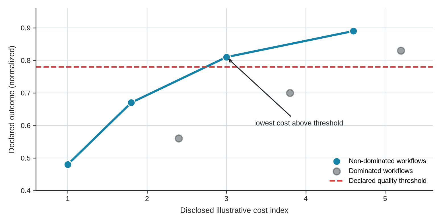
In our physical design workflows, a rapid, inexpensive learned estimate can often stand in for a computationally expensive downstream physical-design analysis (Kahng 2018). Likewise, proposing a clever tool-script change can cost us significantly less than the heavyweight implementation check we need to properly evaluate it. We acknowledge that deploying more expensive upfront reasoning can still be economical if it helps us avoid a large number of failed tool runs, but we must measure this trade-off rather than assume it. We report our design quality as a function of our total cost, we identify the non-dominated points on our cost-quality frontier, and we report the precise cost required to reach our predeclared architectural quality threshold. When we plot our quality directly against our total cost, we preserve the lessons behind simulator-tax and cost-quality plots, all without making the fatal assumption that our AI inference costs and our EDA tool costs will always form one universal, monolithic curve.
Plotting a normalized, predeclared architecture outcome against total resource expenditure turns the cost-quality tradeoff into something we can read directly (Figure 10.1). The non-dominated frontier collects the workflows that achieve the most quality for a given expenditure, while dominated workflows fall below it, spending more total cost without a better supported result. Against a predeclared quality threshold, the frontier identifies the exact resource expenditure a workflow needs to breach that threshold and yield a defensible design recommendation.
Our vertical axis must represent one predeclared architecture outcome, or an explicit, mathematically defined comparison rule for our declared objectives and constraints. We do not use this as an excuse to blur performance, power, area, correctness, and other critical dimensions into an arbitrary, hidden score.
These points are synthetic illustrations. In our real studies, we must plot our measured budgets against our predeclared architecture outcome, show our uncertainty, and preserve our underlying resource vector.
10.5 Matched Baseline and Candidate Comparisons
When we evaluate a program claim, we are asking a pragmatic adoption question. Does embracing the complete workflow improve our supported architecture outcomes or lower our total cost relative to the strongest practical alternative? We evaluate this across a declared set of tasks, conditions, budgets, and checks. We recognize that this adoption standard is stricter than asking if an AI-native system can discover a single valid design. To answer it, we must match our complete workflows. We lock in the same architecture question, starting artifacts, source and evaluation-tool access, evaluator-owned checks, conditions, cost rules, budgets, and stopping rules for both sides. While our competing workflows might rely on wildly different internal procedures, those mechanical differences simply become part of their distinct identity, overarching effect, and total cost.
Deploying distinct comparison arms allows each one to answer a different architectural question. For example, if we use a random or enumerated search baseline, we are testing whether our guided search outsmarts naive sampling. Conversely, when we pit an AI method against a strong conventional or human-directed workflow, we are testing whether our point AI assistance advances current engineering practice. By systematically stepping through a no-AI arm, a retrieval-only configuration, foundation-model assistance, and our fully configured workflow, we reveal exactly how capability and cost scale across the entire system. Because each baseline targets a specific hypothesis, we can never rely on a single baseline to support all our architectural claims.
Random search still holds value for us. It acts as a diagnostic floor that can expose a learned search method performing no better than blind sampling at the same budget constraint. However, we must remember it is purely diagnostic, not a credible alternative a professional architecture team would deploy in production. Depending on our specific architectural task, our true practical alternative might be direct enumeration, a robust deterministic heuristic, a highly tuned commercial or in-house optimizer, an established EDA flow, or a comprehensive human-directed study. As we explain in Chapter 5, we derive our strongest alternative from the represented problem itself, rather than blindly selecting from a fixed hierarchy of methods.
Our comparisons lose meaning the moment we allow one arm to exploit richer starting information, stronger evaluation tools, deeper tuning, or a more forgiving stopping rule. While we acknowledge that those advantages might be legitimate facets of a specialized workflow, we must account for them as part of system identity and total cost rather than letting them be presented as an artificial intelligence breakthrough. Strict matching, held across every listed element (Table 10.6), eliminates alternative explanations and forces comparative gains to reflect complete-workflow performance.
| Comparison element | Matching rule |
|---|---|
| Evaluation object | We compare complete human-plus-technical workflows for our adoption estimate. We reserve method, component, or narrower AI contributions for controlled replacements or ablations. |
| Architecture question | We ask both systems to resolve the exact same decision and preserve identical candidate and condition identities. |
| Starting information | We give both arms the same specifications, starting artifacts, workload information, prior results, and source access, except where access itself is our tested component. We record which sources each system actually consumes. |
| Development and tuning | We grant both arms comparable opportunity, expertise, and budget for prompt, procedure, baseline, heuristic, parameter, and workflow tuning. We always record inherited development effort and explicitly note any remaining asymmetry. |
| Evaluation tools and checks | We give both arms access to the same evaluator-run tools and fidelity stages, judging them with our identical evaluator-owned acceptance checks and criteria. We treat workflow-internal tools and checks as system components, record their cost, and document any arm-specific access. |
| Budget | We enforce a single cost-accounting window and compare at declared human, machine, tool, review, and elapsed-time budgets, preferably spanning several budget points rather than relying on one arbitrary cutoff. |
| Human capability | We deploy practitioners with appropriate task knowledge in both arms and record their specific actions. We recognize that equal clock time does not automatically make unequal engineering expertise comparable. |
| Human-judged outcomes | We conceal arm identities and randomize review order wherever the artifact permits it. We carefully record unavoidable cues, unblinded judgments, reviewer agreement, and our final adjudication. |
| Stopping rule | We apply the exact same success, failure, exhaustion, and timeout conditions across the board. |
| Reporting | We publish the same architecture outcomes, failed runs, costs, and uncertainty profiles for both arms. |
We do not require our workflows to utilize identical internal methods, wrappers, checks, or procedures, because those internal variations fundamentally define the workflow we are evaluating. While our matching discipline strips away alternative explanations for top-level performance, we understand that it does not, and cannot, isolate the contribution of a specific method or component when internal procedures or human effort differ between the arms.
A matched evaluation routes a single declared architecture question and evaluator-owned evidence standard into two parallel arms, our AI-native workflow and our strongest practical alternative (Figure 10.2). A shared matching header fixes the starting artifacts, source access, evaluation tools, acceptance checks, budget windows, and stopping rules before either arm runs, so the arms differ only in the workflow under test: the AI-native arm works through its configured models, tools, and human interventions, and the conventional arm executes the strongest established human or technical baseline. Each arm returns a supported architecture outcome or a declared failure alongside a full resource-cost record, and the task-paired differences across those outputs isolate the total effect of adopting the AI-native workflow without confusing holistic gains with isolated component contributions.
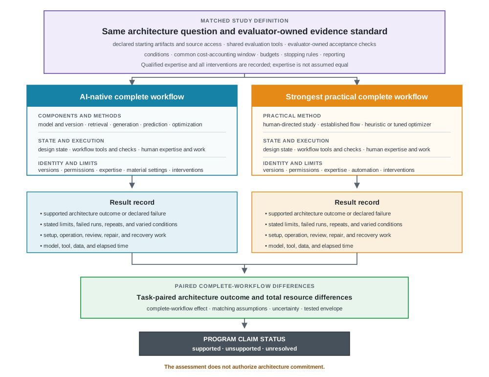
When we share this header, we lock in the architecture question, evidence standard, resource window, and reporting rules before the arms ever diverge. Once launched, each arm returns either a supported outcome or a declared failure, and we log all failed attempts in its record. When we measure the task-paired differences in supported architecture outcomes and total consumed resources, we estimate the complete-workflow impact across repeated runs and varied conditions. Our uncertainty, matching assumptions, and specific tested envelope tightly bound this estimate. If we tolerate any mismatch, we weaken the estimate’s integrity. If our goal is to isolate a specific method or component, we must pivot to the controlled replacements discussed in the next section.
Our architecture-result and total-cost definitions now apply symmetrically to both arms. Generating a cheap, invalid design is never a cost win. When we adhere to matched comparisons, we estimate the complete-workflow effect. From there, we rely on controlled replacements to locate the exact methods and components upon which that workflow effect depends.
Long before we let either arm execute a single run, we predeclare our primary architecture outcomes, required task and condition coverage, acceptable total-cost envelope, and the minimum thresholds for worthwhile architecture improvement and cost reduction. We also establish a strict limit on the maximum acceptable architecture-quality loss. We explicitly state exactly how many paired tasks and statistical repeats we need to distinguish those precise margins with any useful confidence. If we neglect these rules, we risk falling into the trap of analyzing the data post-hoc, retroactively classifying an imperceptible gain as successful, or justifying a cheaper result even when the underlying architecture quality has materially degraded.
We bake our task population and sampling rules into the study plan. First, we name the exact class of architecture decisions our program claim covers. Then, we state how we will sample our tasks, workloads, implementation conditions, and repeats from that defined class. When we engage in adaptive prompt development, method tuning, and search heuristics, we confine that work to a designated development set. For our primary program comparison, we insist on using held-out tasks and conditions that never influenced our design choices. Finally, we lock in our findings with an evaluator-owned confirmation of any selected architecture result.
We maintain a firewall between our exploratory configuration development and our confirmatory evaluation (Nosek et al. 2018). The record states how many prompts, models, routing policies, metrics, task variants, and analysis techniques we evaluated before settling on the final comparison. We name our primary outcome and target analysis before inspecting the holdout set. If adaptive searching across various configurations or outcomes could plausibly explain our reported advantage, we demand a fresh confirmation set rather than treating the best-selected result as confirmatory (Dwork et al. 2015). We apply this exact same development opportunity and stringent accounting rule to our strongest practical alternative. Even if a mature baseline carries decades of inherited tuning, our study must record that historic advantage rather than tuning only the AI-native arm and falsely declaring the final contest matched.
Nosek, Brian A., Charles R. Ebersole, Alexander C. DeHaven, and David T. Mellor. 2018. “The Preregistration Revolution.” Proceedings of the National Academy of Sciences 115 (11): 2600–2606. https://doi.org/10.1073/pnas.1708274114.
Whenever human engineers direct either arm, we assign their tasks using a predeclared balancing or randomization rule, logging who worked on which task. If we have the same architect operate both systems, we rotate the tool order and account for any design knowledge carried over from the first arm into the second. If we deploy different engineering teams, we match their relevant experience and report any remaining skill gaps. We do not pretend these controls make human expertise identical; rather, they make our human comparison mathematically interpretable. We provide both arms with a declared familiarization period and a thoroughly stable operating procedure, strictly separating that setup time from our measured task duration. If exposure to the first arm reveals critical design insights that would unfairly advantage the second, we force the use of fresh tasks, implement a declared washout period, or apply an analysis that explicitly models the cognitive carryover.
Whenever an outcome is human-judged, like hardware maintainability or the quality of an architectural explanation, we hide the arm labels and randomize our review order wherever feasible. We acknowledge that some generated artifacts inevitably reveal their origin through distinct coding styles or structural quirks. In those cases, we honestly record those leaked cues, any resulting unblinded judgments, our reviewer agreement rates, and our final adjudication procedures, rather than falsely claiming a perfect blinding protocol that our evaluators could not maintain.
We demand that every assigned run remains in our final result pool. If an architecture run yields an incomplete design, triggers a timeout, suffers a tool failure, or exhausts its compute budget, it still receives its declared result status and resource cost. We never let failed runs quietly disappear just because they failed to produce a final benchmark score. While we can report results restricted to successful runs as a secondary, optimistic view, we never allow them to replace the all-assigned comparison upon which our entire program claim depends.
We treat a timeout as a failure when our targeted outcome is success within a fixed budget. However, we treat it as a right-censored event when our outcome metric is simply the time required to reach a supported result; in that scenario, the true completion time is mathematically known only to exceed the timeout threshold. As we introduced in Chapter 4, this is the classic timeout-specific form of a censored observation. Our analysis must never discard either case, nor can we assign a fabricated completion time just to make the math look cleaner.
We apply the cost-quality comparison from Figure 10.1 to both arms across several predeclared budget milestones. As human effort, model compute, tool utilization, and elapsed wall-clock time increase, we report the best supported architecture outcome at each step, alongside the total overarching cost required to breach our declared quality threshold. We enforce the resource-envelope or disclosed-conversion rules we established in the total-cost section. Two divergent resource vectors are never equivalent just because an author summarized both as “cost.”
10.6 Evaluating Workflow-Level Design Effects
Evaluating an AI-native workflow using a matched strongest-practical comparison measures the impact of adopting the entire system. However, this high-level view obscures which architectural component or method drove the performance gains. To pinpoint where the value lies, we rely on controlled replacements and ablations. When we swap out or remove a single core element, while holding the surrounding system architecture, human procedures, task definitions, verification checks, and hardware budgets constant, we isolate its impact. Targeted single-element substitutions (Table 10.7) isolate internal dependencies within our workflow without falsely assuming component contributions are purely additive.
| Component under test | Useful comparison | Claim the comparison can support |
|---|---|---|
| Complete AI-native workflow | Compare with the strongest practical alternative workflow under the same task, evidence standard, and total-cost accounting | The effect of adopting the whole workflow on result quality or cost, not an isolated AI contribution |
| Foundation model | Replace it with retrieval-only assistance, a smaller model, or another declared model while preserving the surrounding workflow | Whether the measured result depends on that model capability and its cost |
| Generation | Replace generated candidates with the same-size human, rule-based, or existing candidate set | Whether generation changed candidate quality or diversity at the declared cost |
| Prediction | Remove the learned screen or replace it with a conventional proxy and send a matched sample to the higher-fidelity check | Whether prediction saved evaluation work without discarding decisive candidates |
| Optimization | Replace the search policy with the strongest practical conventional method at matched budgets | Whether the optimizer improved the cost-quality relationship |
| Retrieved design information | Remove, freeze, or substitute the retrieval source while preserving the remaining system; check source versions, decision-relevant coverage, conflicts, and local claim support | Whether retrieved material changed results and which source dependencies remain |
| Routing and role selection | Replace adaptive routing with a fixed sequence or evaluator-declared component choice | Whether dynamic method and tool selection improved decisions or merely added complexity |
| Tool feedback | Restrict or delay selected feedback attributes while keeping tool stages fixed | Which returned information enables correction and which merely adds cost |
| Automated checking | Replace one checker with an independently developed check where feasible | Whether the conclusion depends on one checker or one shared assumption |
| Human intervention | Compare declared intervention policies and record every intervention | How much human work is necessary for the measured result |
Whenever we want to evaluate the quality of a new architectural method, we must equalize our tool budgets. Conversely, when our goal is to measure the end-to-end efficiency of the complete workflow, we can let the budgets vary, provided we account for every resource spent. Any claim we make must remain bounded to the specific component or entire workflow that we modified in our comparison.
We cannot assume that one-at-a-time replacements guarantee causal isolation, because architectural components interact. For instance, a specific predictor may only operate effectively when paired with a particular hardware optimizer, or a foundation model might seem capable only because a human designer silently patches its flawed tool calls. In practice, our evaluations must start by isolating the components most likely to drive the observed performance gains. We then test targeted interactions when our initial conclusions shift, transparently reporting any tightly coupled dependencies we cannot cleanly separate. Whenever complex interactions with software wrappers, verification checks, manual procedures, or human oversight thwart our attempts at isolation, we must concede that the individual component’s contribution remains unresolved. Architectural contributions are rarely additive; we cannot reconstruct the total performance gain of a complex system by summing the isolated, one-at-a-time deltas of its interacting parts.
Given a large design space where dozens of architectural components interact, we often turn to preregistered fractional-factorial experiments to screen a balanced subset of configurations, sparing us the impossible task of enumerating every combination. For an efficient first-pass screen of main effects, we frequently rely on Plackett-Burman designs (Plackett and Burman 1946). Once we complete that initial sweep, we can deploy targeted designs to untangle specific, high-value interactions. However, even the most promising subsystem combinations demand held-out confirmation against our own evaluator-owned architectural benchmarks. Screening inherently aliases main effects with deeper interactions and never makes component contributions additive. Consequently, any untested or inseparable hardware interactions will remain unresolved in our final analysis.
Plackett, Robin L., and J. Peter Burman. 1946. “The Design of Optimum Multifactorial Experiments.” Biometrika 33 (4): 305–25.
Isolating a component’s contribution is merely our first hurdle. Our next challenge is proving that the complete-workflow improvements, and the specific component dependencies driving them, recur across the same task and survive the real-world architectural conditions our claims cover.
10.7 Reliability Across Environmental Operating Conditions
Even if we estimate a favorable outcome and cost difference, that alone does not guarantee a reliable architectural advantage. When we run our workflows repeatedly, we can verify whether a desired effect recurs on the same task. However, to understand whether an advantage survives the practical shifts inherent in any architecture decision, we must also test it under varied conditions. We need both forms of evidence to build confidence in our designs; a single stochastic run is merely an anecdote, not a measurement (Henderson et al. 2018).
Henderson, Peter, Riashat Islam, Philip Bachman, Joelle Pineau, Doina Precup, and David Meger. 2018. “Deep Reinforcement Learning That Matters.” Proceedings of the AAAI Conference on Artificial Intelligence 32 (1): 3207–14. https://doi.org/10.1609/aaai.v32i1.11694.
For us, reliability must mean more than achieving an acceptable average success rate. A reliability report covers our worst-case scenarios, any blocking constraint violations we encounter, and our mechanisms for recovery after a failure. We must also quantify the time and human effort required for that recovery, alongside the fraction of automated decisions our experts ultimately override. We need to test whether our reported confidence levels calibrate with our eventual architectural results. Consider a workflow that is correct 90 percent of the time but expresses maximum confidence during its most catastrophic failures. This presents a different engineering risk profile compared to a workflow with the identical pass rate but properly calibrated uncertainty estimates.
While our earlier decision-quality tests establish our confidence in overall workflow outcomes, our numerical architecture estimates demand their own calibration record. We must report our interval coverage, our interval sharpness (ensuring narrowness without sacrificing coverage), and any errors present near our decision boundaries (Gneiting and Raftery 2007, 369, 374). We must tie each of these metrics to a specific tool stage, time horizon, and condition distribution. We cannot assume that calibration on one specific workload, process node, design family, or toolchain will hold once any of those conditions shift. Much like predictive-uncertainty evaluations in machine learning demonstrate degradation under dataset shift (Ovadia et al. 2019), an architecture predictor faces similar perils. When we change a workload, process node, design family, or toolchain, we introduce a new target condition. We must then measure our interval coverage and error all over again. This testing only qualifies our predictor’s uncertainty under that newly defined condition; it does not prove that our proposed architecture is functionally correct or physically feasible.
Gneiting, Tilmann, and Adrian E. Raftery. 2007. “Strictly Proper Scoring Rules, Prediction, and Estimation.” Journal of the American Statistical Association 102 (477): 359–78. https://doi.org/10.1198/016214506000001437.
Ovadia, Yaniv, Emily Fertig, Jie Ren, et al. 2019. “Can You Trust Your Model’s Uncertainty? Evaluating Predictive Uncertainty Under Dataset Shift.” Advances in Neural Information Processing Systems 32: 13991–4002. https://proceedings.neurips.cc/paper_files/paper/2019/hash/8558cb408c1d76621371888657d2eb1d-Abstract.html.
10.7.1 System Variance
When we set up our evaluations, we should carefully pair our comparison arms across tasks, controlled tool factors, and declared starting conditions. We must treat changes to model or search seeds as repeated runs under a single, fixed system configuration. Conversely, we should view a changed prompt as an altered system configuration, unless a predeclared prompt-sampling policy is defined as part of the system we are testing. None of these variations constitute an independent architecture task. As we analyze our data, we should report successes, failures, constraint violations, recoveries, medians, interquartile ranges, and granular per-task results. We must avoid relying solely on means and standard deviations, as they can mask the reality of hardware studies that exhibit bimodal outcomes, situations where one cluster of runs fails implementation while another discovers a strong design.
Our evaluation apparatus itself introduces another layer of variability. For instance, subtle shifts in placement seeds and tool settings can alter our physical-design fit (Altera 2026a), while supposedly neutral build or environment adjustments can perturb our measured performance (Mytkowicz et al. 2009). To ensure our nominally fixed setups are repeatable, we must conduct identical reruns. From there, we can employ separate sensitivity studies to deliberately vary specific factors. We must never subtract environmental variance from our model variance under the false assumption that they are automatically independent. Instead, we should predeclare exactly what our comparison is estimating. Are we looking at an average across declared apparatus factors, a result frozen at one specific setup, or a true worst-case scenario? We must estimate that targeted quantity, and its interval, using a study design that isolates these factors whenever possible. If we find that the system differences cannot be distinguished from the noise induced by our apparatus at our required practical margins, we must accept that our architectural result remains unresolved.
Altera. 2026a. SEED: Quartus Prime Pro Edition Settings File Reference Manual. https://docs.altera.com/r/docs/683296/25.3/quartus-prime-pro-edition-settings-file-reference-manual/seed.
Mytkowicz, Todd, Amer Diwan, Matthias Hauswirth, and Peter F. Sweeney. 2009. “Producing Wrong Data Without Doing Anything Obviously Wrong!” Proceedings of the 14th International Conference on Architectural Support for Programming Languages and Operating Systems (ASPLOS), 265–76. https://doi.org/10.1145/1508244.1508275.
Chen, Mark, Jerry Tworek, Heewoo Jun, et al. 2021. “Evaluating Large Language Models Trained on Code.” arXiv Preprint arXiv:2107.03374, ahead of print. https://doi.org/10.48550/arXiv.2107.03374.
Jimenez, Carlos E., John Yang, Alexander Wettig, et al. 2024. “SWE-bench: Can Language Models Resolve Real-World GitHub Issues?” International Conference on Learning Representations (ICLR). https://doi.org/10.48550/arXiv.2310.06770.
pass@k can describe whether at least one out of \(k\) generated candidates for a given task achieves a binary pass. When we use it, we must report our underlying estimator and sampling conventions (Chen et al. 2021; Jimenez et al. 2024). In hardware design, however, this metric requires a strict time or tool budget; finding a single success buried among dozens of expensive failures is often practically useless for our pipelines. When we evaluate true deployment reliability, we are asking a different question. How often does an ordinary, everyday run succeed? We are not asking if brute-forcing enough attempts eventually yields a winner. Neither of these scores tells us anything about physical validity beyond the narrow definition of the check we used to define a “pass.”
Our statistical analysis must align with both our raw data and our ultimate architectural claims. While paired comparisons prove useful when we evaluate competing systems across identical tasks and conditions, the corresponding nonparametric tests still rely on paired observations and independent task units (Demšar 2006). We can leverage bootstrap intervals (drawing paired experimental units with replacement to estimate statistic variation (Efron and Tibshirani 1993)) to summarize highly skewed statistics, but generating additional resamples will never remedy a small, unrepresentative task set. We should report our realized sample sizes, observed failures, effect sizes, calculated intervals, and the rationale behind our specific analysis choices, rather than treating any single statistical test as universally mandatory.
Demšar, Janez. 2006. “Statistical Comparisons of Classifiers over Multiple Data Sets.” Journal of Machine Learning Research 7 (1): 1–30. https://www.jmlr.org/papers/v7/demsar06a.html.
Efron, Bradley, and Robert J. Tibshirani. 1993. An Introduction to the Bootstrap. Vol. 57. Monographs on Statistics and Applied Probability. Chapman & Hall.
Agarwal, Rishabh, Max Schwarzer, Pablo Samuel Castro, Aaron C. Courville, and Marc G. Bellemare. 2021. “Deep Reinforcement Learning at the Edge of the Statistical Precipice.” Advances in Neural Information Processing Systems 34: 29304–20. https://proceedings.neurips.cc/paper/2021/hash/f514cec81cb148559cf475e7426eed5e-Abstract.html.
When our studies claim generalized performance across a broad task population, we must treat our core architecture tasks as our primary generalization units. We should pair our systems within specific tasks and conditions, and we must treat our repeated runs strictly as nested observations rather than independent, extra tasks (Agarwal et al. 2021). A fixed, finite benchmark suite or a simple convenience sample supports nothing beyond the narrow population it represents. We need to detail our per-task effects, uncertainty bounds, failure rates, and practical decision margins, reporting an aggregate across-task effect only when our sampled task population justifies it. We must keep our exploratory configuration tuning separated from our held-out confirmation testing, and we should declare how evaluating multiple outcomes or engaging in subgroup comparisons ultimately impacts our final decision rules.
10.7.2 Operating Condition Sweeps
Whenever we conduct a scaling study, we must name the architectural difficulty axis we are probing. We can use axes such as the total legal design-space size, the number and coupling of our constraints, the depth of our tool-flows, our feedback costs, or our cross-layer span. Against whichever axis we choose, we should report our supported outcomes, failures, required human interventions, overall reliability, and total resource costs. While we might adjust model sizes and task counts as convenient experimental settings, neither of these adjustments establishes that our core architectural problem became harder.
Sweeping operating conditions tests whether a complete-workflow advantage remains stable or collapses outside a narrow environment envelope; the condition-variation matrix declares which axes we sweep and which we hold fixed (Table 10.8).
| Factor family | Conditions to vary | Comparison basis held fixed | Question the variation answers |
|---|---|---|---|
| Workload and software | Input distribution, workload phase, compiler, runtime, and mapping | Architecture question, candidate identities, evaluator-owned checks, and total-cost rule | Does our complete-workflow advantage survive beyond a single workload or specialized software path? |
| Architecture and system | Interface traffic, memory hierarchy, synchronization, and energy assumptions | Required functions, declared objectives, workflow identities, and acceptance rules | Does our localized gain remain useful after we represent the surrounding system costs? |
| Implementation and tools | Fidelity stage, physical corner, tool version, configuration, and seed | RTL intent, acceptance properties, comparison arms, and resource-accounting window | Does our advantage survive higher-fidelity checks and inevitable apparatus variation? |
| Workflow configuration and information | Prompt or instruction policy, model or routing configuration, retrieval source, and represented-state freshness | Task population, legal actions, evaluator-owned tool access, checks, and reporting rules | Does our advantage depend entirely on one brittle configuration or a stale information state? |
When we observe an advantage disappearing, it narrows our tested envelope. We use this matrix to map our boundaries, not to decide what concepts will transfer to a new design program; we explore the separate, complex question of reuse across new targets deeply in Chapter 9.
We can never allow a single isolated task to support a sweeping, program-wide claim. To be useful, our evaluation suite must span distinct architecture decisions, diverse workloads, varied designs, fluctuating result costs, multiple representations, different tool stages, and a wide range of failure consequences. We must transparently report the precise envelope in which our architectural advantage repeats, the exact conditions where it evaporates, our absolute worst observed cases, and the specific scenarios we opted not to test. Also, we need to report whether we detected failures before an invalid candidate advanced deeper into the pipeline, and whether our automated workflows successfully recovered without requiring expert repair. This is how we achieve empirical generalization; producing similar-looking artifacts is never enough for hardware design.
As we synthesize our results, we must keep four levels of claims distinct. First, our repeated runs solely measure stochastic behavior on the exact same task. They simply show us whether our identically configured workflow repeats its outcome; they do not prove that our outcome survives a changed task or an altered system environment.
Second, we define robustness as absolute stability under declared, meaning-preserving changes that theoretically should not alter our correct architecture results. As architects, we deliberately perturb an input encoding, a seed, a representation spelling, or an apparatus setting while preserving the underlying task. We then verify whether our supported results, constraint statuses, and recovery behaviors remain strictly within our predeclared limits. If we encounter a failure during this process, it correctly narrows our broader conclusions down to only the conditions that remained provably stable. If we instead change a prompt, alter representation semantics, or shift our tool policies, we are no longer testing robustness; we are essentially defining a different system.
Third, we use held-out tasks to support generalization within a declared design population, but this only holds when our sampling or selection represents that specific population and those tasks remained cordoned off from our system and evaluator selection phases. A simple convenience holdout is not validation; it is merely an unseen data point.
Finally, whenever we introduce a new design family, toolchain, process node, organization, or decision class, we create a transfer claim that demands a new target evaluation. We must re-estimate our performance and calibration at each of these new levels. We have to treat any untested change as a hard boundary on our evaluation claims. When we do choose to cross factor families, such as mixing a specific workload with a new compiler, or a novel design with a harsh physical corner, we must do so deliberately, specifically because their underlying interaction forms part of our architectural risk model.
An architectural result bounded to a single tested envelope remains meaningful and comparable only when our benchmark’s underlying tasks, rules, and reporting structures support comparison against other complete workflows.
10.8 Benchmark Health, Contamination, and Standardization
While benchmarks provide the foundation for repeatable comparisons, they can never replace sound architectural judgment. In our work, we use benchmarks to map metrics against a strictly defined task, a permitted action space, and a specific depth of evidence. We know that standard suites like SPEC CPU, PARSEC (a shared-memory parallel benchmark suite), and MLPerf succeeded because they established shared workloads, explicit rules, and standard reporting conventions that allowed our community to meaningfully compare results (Bienia et al. 2008; Standard Performance Evaluation Corporation 2017; Mattson et al. 2020). For AI-native architecture, our benchmarks must go further. We have to define both the design challenge and the autonomous system permitted to solve it. Any resulting score serves merely as a single instrument within our broader workflow evaluation.
Bienia, Christian, Sanjeev Kumar, Jaswinder Pal Singh, and Kai Li. 2008. “The PARSEC Benchmark Suite: Characterization and Architectural Implications.” Proceedings of the 17th International Conference on Parallel Architectures and Compilation Techniques, October, 72–81. https://doi.org/10.1145/1454115.1454128.
Standard Performance Evaluation Corporation. 2017. SPEC CPU 2017 Benchmark. https://www.spec.org/cpu2017/.
Mattson, Peter, Vijay Janapa Reddi, Christine Cheng, et al. 2020. “MLPerf: An Industry Standard Benchmark Suite for Machine Learning Performance.” IEEE Micro 40 (2): 8–16. https://doi.org/10.1109/MM.2020.2974843.
Liu, Mingjie, Nathaniel Pinckney, Brucek Khailany, and Haoxing Ren. 2023. “VerilogEval: Evaluating Large Language Models for Verilog Code Generation.” IEEE/ACM International Conference on Computer-Aided Design (ICCAD). https://arxiv.org/abs/2309.07544.
Lu, Yao, Shang Liu, Qijun Zhang, and Zhiyao Xie. 2024. “RTLLM: An Open-Source Benchmark for Design RTL Generation with Large Language Model.” Proceedings of the 29th Asia and South Pacific Design Automation Conference (ASP-DAC). https://arxiv.org/abs/2308.05345.
Wang, Chenyu, Zishen Wan, Jeffrey Ma, et al. 2026. ArchEval: Measuring AI Agents as Computer Architects. arXiv preprint arXiv:2607.03601. https://arxiv.org/abs/2607.03601.
Wang, Zhihai, Zijie Geng, Zhaojie Tu, et al. 2025. “Benchmarking End-to-End Performance of AI-Based Chip Placement Algorithms.” Advances in Neural Information Processing Systems 38. https://proceedings.neurips.cc/paper_files/paper/2025/hash/1cba8502063fab9df252a63968691768-Abstract-Datasets_and_Benchmarks_Track.html.
Zhou, Peilong, Zhirong Chen, Cangyuan Li, et al. 2026. CLOSER-Bench: Evaluating Budgeted Cross-Stage Design Closure for Hardware Agents. https://doi.org/10.48550/arXiv.2607.16632.
Tsai, Pei-Huan, Kuan-Lin Chiu, William Baisi, Pin-Yu Chen, and Luca P. Carloni. 2026. HSCO-Bench: An Agent-Driven End-to-End Hardware-Software Co-Design Benchmark for Systems-on-Chip. https://doi.org/10.48550/arXiv.2605.19399.
When we look at existing benchmark suites, we see a progression of evidence depth rather than a simple catalog of tests. At the functional RTL level, VerilogEval tests whether our generated Verilog works as intended (Liu, Pinckney, et al. 2023), while RTLLM pushes further by measuring post-synthesis quality of results (Lu et al. 2024). ArchEval gives us the ability to record design trajectories under specific simulator configurations and harness settings (C. Wang et al. 2026). Taking this into the physical domain introduces different constraints; ChiPBench, for example, evaluates placement methodologies through a standardized physical flow (Zhihai Wang et al. 2025). We can push the evidence even deeper through cross-stage analysis and deployed evaluations. CLOSER-Bench bridges the gap between simulation, synthesis, static timing, and place-and-route to weigh the costs and recoveries of our tools, while HSCO-Bench targets full FPGA-deployed SoC prototypes on specific platforms (Zhou et al. 2026; Tsai et al. 2026). With each progressive step, we introduce distinct tools, checks, costs, and claim boundaries. However, our results remain bounded by the deepest stage we successfully complete. No single suite can prove that our complete AI-native workflow outperforms credible alternatives across an entire architecture program.
10.8.1 Pinning Action Spaces
We can only interpret a benchmark score when its release pins down the task, the permissible actions, the validation checks, and the depth of evidence. We should carry over the frozen system and environment identity that we outlined in Table 10.1, and then layer on the following benchmark-specific elements:
- the benchmark version, task and split identifiers, our sampled architecture population, and the clear boundaries separating development, holdout, and confirmation datasets;
- the hidden tests owned by our evaluators, the specific information and feedback we expose to the system, and any permitted changes specific to the benchmark;
- the rules we use for scoring, aggregation, failure, censoring, and repeated submissions; and
- our records of contamination, refresh policies, and criteria for retiring outdated tasks.
The system under test must never be allowed to alter our evaluator-owned requirements, rejection criteria, or scoring rules. If modifying a constraint, testbench, or tool script happens to be the architectural task, we must rely on an independent, evaluator-controlled check to verify that the proposed changes remain legal and valid.
How we select our tasks determines what our benchmark represents. We must eliminate exact and near-duplicate tasks across our development and evaluation splits. Rather than generating dozens of trivial variants for a single easy hardware block, we need to preserve distinct design families and explicitly state the architecture population our suite aims to sample. We should maintain hidden tests and evaluator-owned holdouts for properties that we do not want systems optimizing directly. However, we must document the categories and failure rules for these hidden tests thoroughly enough so that the task remains an engineering problem, not a frustrating guessing game.
Benchmark validity is an inference connecting tasks to a claim; it is never an intrinsic property of the score itself. To make this inference concrete, we should ask three questions. Do our evaluator-owned checks actually measure success on the specified task? Does the score genuinely reflect the claimed architectural capability, or is it merely rewarding syntax repair, test harness familiarity, or checker exploitation? Do the task distributions, design artifacts, feedback loops, compute budgets, and human interactions mirror the real-world design programs where we intend to apply these results? To ensure clarity, we must construct a claim-to-task map that links each program claim to our sampled design decisions, failure consequences, and stages of evidence. Any gaps in this map must be treated as explicit limits on our claims, rather than brushed aside as hidden assumptions.
Our architectural claims are always bounded by the deepest evaluation stage we complete. We must report the specific stage, the identity of the checks performed, the outcome categories, the computational cost, the coverage metrics and waiver statuses, as well as the flow of our candidates. Once we report these details, we apply the check-specific scope outlined in Chapter 7. Passing an early stage only supports the narrow claims that specific stage is capable of testing.
The depth of our evidence dictates our evaluation costs. It is inefficient to push malformed RTL through a lengthy, expensive physical design flow. We can certainly design our benchmarks to run cheap checks before executing computationally intensive ones, but we are obligated to report exactly which candidates survived to reach each subsequent stage. A cheap proxy score must never be reported as if it came from a physical check. We can leverage state checkpoints to mitigate repetitive setup costs, provided we give all evaluated systems equivalent access and carefully include the restored tool states in our system records. When we cache results, we must key them to our complete environment manifest, not just the RTL hash, because any tweak to a constraint, standard cell library, floorplan, activity file, or tool version constitutes a different architectural evaluation.
As evaluators, we also need to test our own apparatus. We must seed our benchmark releases with deliberately chosen known-good and known-bad designs, apply differential testing to our checkers, and inspect any disagreements that arise between our simulators, formal verification tools, synthesis engines, and physical-design stages. A subtle checker bug or a clever simulator exploit can make an invalid candidate appear capable. We must treat benchmark and tool failures as primary results, openly correct any affected scores, and issue properly versioned releases of our repaired infrastructure.
10.8.2 Benchmark Contamination
RTL-Repo provides 4,098 hardware samples pulled from 1,361 public repositories (Allam and Shalan 2024). Because of this widespread availability, our public benchmark tasks risk significant overlap with the training data of our models (Zeng Wang et al. 2025). When we have access to the training corpus, we can use exact and approximate overlap searches to flag obvious reuse. However, when that corpus is kept hidden from us, our evaluations must state this limitation rather than falsely claiming our benchmarks are free of contamination.
Allam, Ahmed, and Mohamed Shalan. 2024. “RTL-Repo: A Benchmark for Evaluating LLMs on Large-Scale RTL Design Projects.” 2024 IEEE LLM Aided Design Workshop (LAD), 1–5. https://doi.org/10.1109/LAD62341.2024.10691810.
Wang, Zeng, Minghao Shao, Jitendra Bhandari, et al. 2025. VeriContaminated: Assessing LLM-Driven Verilog Coding for Data Contamination. https://doi.org/10.48550/arXiv.2503.13572.
Jain, Naman, King Han, Alex Gu, et al. 2025. “LiveCodeBench: Holistic and Contamination Free Evaluation of Large Language Models for Code.” International Conference on Learning Representations (ICLR). https://arxiv.org/abs/2403.07974.
We can look to LiveCodeBench to see how time-split tasks help reduce exposure to benchmark material (Jain et al. 2025). The lesson for our architecture community is that we must reserve tasks created strictly after an evaluated model’s snapshot date, and then prevent those results from guiding any system configuration before the final evaluation. We must also acknowledge the limitations of borrowing ideas from software. A software-code benchmark simply does not stress our hardware tool flows, enforce physical design constraints, run costly cycle-accurate simulations, or demand complex cross-layer architectural decisions. While keeping private held-out designs and crafting new architecture problems gives us barriers against contamination, we have to admit that none of these methods can prove a model has never encountered our design or one of its close relatives.
We must also be vigilant about private tasks leaking through repeated evaluations. We need to track how often the system, its developers, or its prompt-tuning mechanisms observe our held-out scores and diagnostic feedback. To protect our benchmarks, we should restrict query budgets, limit the granularity of the feedback we return, separate development access from final evaluation runs, and continuously rotate our holdout sets to prevent repeated submissions from reverse-engineering the evaluator. As we know, a private split essentially degrades into development data the moment its feedback is repeatedly used to tune configuration choices (Dwork et al. 2015).
Dwork, Cynthia, Vitaly Feldman, Moritz Hardt, Toniann Pitassi, Omer Reingold, and Aaron Roth. 2015. “The Reusable Holdout: Preserving Validity in Adaptive Data Analysis.” Science 349 (6248): 636–38. https://doi.org/10.1126/science.aaa9375.
While we can use semantics-preserving variants to test a model’s sensitivity to surface-level changes, we must be careful, as arbitrarily renaming meaningful hardware signals or restructuring the RTL can inadvertently alter the architectural task. We rely on functional simulation, formal equivalence checking (where its assumptions hold), and stringent implementation checks to determine if an output satisfies our design requirements. Unfortunately, passing these checks tells us nothing about whether the model solved the problem or regurgitated a memorized solution.
As benchmark maintainers, we carry the responsibility to publish any known corpus overlaps and maintain a firewall between our public development tasks and private evaluation sets. We must record both model and benchmark timestamps, disable any unreported retrieval mechanisms during held-out testing, regularly refresh our holdout pools, and root out near-duplicate tasks. Finally, we must always qualify our architectural conclusions by acknowledging the remaining risks of data exposure.
Even without a single leaked training example, our benchmarks can still suffer from decay. Once our discipline repeatedly optimizes against a static target, the resulting scores often cease to measure the underlying capability we care about. Computer architecture provides us with a durable example of this phenomenon. SPEC deliberately dropped the matrix300 workload from its 1992 suites because a legal compiler optimization exerted an outsized, distorting influence on the final SPEC ratio (Weicker 1995; Hennessy and Patterson 2017, 61, 62).
Weicker, Reinhold. 1995. Answers to Frequently Asked Questions about SPEC Benchmarks. https://netlib.org/performance/html/specfaq.html.
Hennessy, John L., and David A. Patterson. 2017. Computer Architecture: A Quantitative Approach. 6th ed. Morgan Kaufmann.
Therefore, we must establish a complete lifecycle for an architecture benchmark long before its first score is quoted. We need to version each release, cultivate a robust refresh pool, and constantly monitor our suites to see if task success has saturated or if the results have become dominated by narrow, benchmark-specific tricks. We must also define and publish clear retirement criteria. While aging tasks may no longer support bold comparative claims about architectural capability, they can still serve us well as foundational regression tests.
10.8.3 Standardized Reports
When sharing our evaluations, we must publish per-task results before presenting any high-level suite summaries. When we normalize ratios across positive-valued tasks that share a common direction, we should consistently employ a geometric mean rather than an arithmetic mean; the geometric mean remains robustly invariant to our choice of a common reference point (Fleming and Wallace 1986). We must define clear failure policies for invalid runs, zero scores, signed timing slacks, and heterogeneous raw quantities, rather than haphazardly forcing them into an average. Often, our multi-objective architecture outcomes will not admit a single defensible aggregate score. In those situations, we should report constraint pass rates, isolated per-objective results, and non-dominated Pareto sets instead of contriving a weighted score that obfuscates the underlying design tradeoffs.
Fleming, Philip J., and John J. Wallace. 1986. “How Not to Lie with Statistics: The Correct Way to Summarize Benchmark Results.” Communications of the ACM 29 (3): 218–21. https://doi.org/10.1145/5666.5673.
To ensure our reporting remains comparable, we must reuse the frozen identities and cryptographic hashes we established in Table 10.1. To this foundation, we should add the specific benchmark versions, task and split identifiers, random seeds, compute budgets, stopping criteria, failure rules, aggregation policies, and the exact scripts required to regenerate our summaries from the raw data. We must preserve enough candidate and attempt records so that our peers can investigate anomalous or invalid scores without forcing anyone to disclose proprietary design data. If our results rely on a private hardware design, a confidential process design kit (PDK), or a proprietary EDA tool, we are obligated to explicitly name that inaccessible boundary and, wherever feasible, provide an alternative public validation path.
We can supplement our per-task and per-objective results by incorporating trajectory measures. Consider integrating the following into our analysis:
- tracking the best supported outcome against total cost, which reveals how rapidly our system converges on useful architectural results;
- logging proposals and failures categorized by tool stage, allowing us to expose exactly where the system squanders expensive evaluations;
- analyzing corrections made after a returned failure, demonstrating whether our next action actually resolves the issue without triggering a new disqualifying violation;
- monitoring repeated states and recurring failure classes to pinpoint areas of ineffective iteration within our design loops; and
- measuring proxy fidelity on an independently selected audit sample near the critical decision boundary, which proves whether our cheaper screening models accurately retained and ordered the test cases that mattered.
We must treat these trajectory metrics as diagnostics, not as definitive evidence of underlying reasoning capabilities. If we want to compute the area under a trajectory curve, we have to establish a declared cost axis, a common starting point and horizon, directionally consistent normalization, robust rules for feasible candidates, and a unified treatment for failures, timeouts, and censored runs before we can even begin to compare two values. We should also recognize that a “best-so-far” curve is monotonic by construction; it tells us nothing about whether the underlying search path thrashed before finding a solution. Monotonic improvement is not a requirement in our multi-objective design spaces. An effective architectural exploration might need to temporarily regress on one metric just to maneuver into a superior design region.
Once our benchmark succeeds in making ordinary baseline comparisons reproducible, we must subject it to deliberate challenges. We have to continually ask ourselves whether these comparisons remain trustworthy when our underlying architectural assumptions, tool interfaces, and validation checks are attacked.
10.9 Red-Teaming AI Hardware Generation Workflows
We elevate red-teaming hardware workflows into a foundational principle for architectural evaluation, deploying structured adversarial attacks against our own design methodologies, tool interfaces, and constraint handlers to expose hidden vulnerabilities before silicon commitment. Rather than passively waiting for failure, we deploy adversarial strategies to break our workflows, hardening our AI-native systems against both malicious exploitation and systemic collapse.
When we perform ordinary evaluation, we ask how our architecture framework performs under expected conditions. Red teaming forces us to confront the opposite scenario. We must ask what happens when our core assumptions vanish, when malicious inputs infiltrate our workflow, when tool feedback actively misleads our search, or when our scoring functions incentivize optimizing a design by quietly weakening the original constraints. Our goal here is not merely to tabulate a generalized “security score.” Instead, we aim to expose concrete, architectural failure classes and measure our ability to detect, interrupt, correct, and recover from them, while quantifying our residual uncertainty. We select tests that challenge both the final emitted hardware design and the automated workflow that generated it.
We must distinguish among red teaming, fault injection, and robustness stress, as they serve different diagnostic purposes and require distinct success conditions in an architecture context. In a red-team test, we grant a declared adversary a highly specific path to manipulate a critical asset or system authority. Our evaluator-owned checks then take over to determine whether our workflow flags the invalid microarchitectural candidate, halts the attack vector, contains any downstream effects, and supports a full state recovery. Passing such an evaluation applies to that single, tested access path and attack scenario.
In contrast, nonmalicious fault injection deliberately triggers specified EDA toolchain or infrastructure failures, such as simulator timeouts, truncated timing reports, or unexpectedly dropped software licenses. We then record exactly how our design workflow recovers from these disruptions. FATE and DESTINI provide a strong systems precedent for deploying such orchestrated faults to stress-test complex recovery paths (Gunawi et al. 2011).
Robustness stress takes yet another approach. We systematically vary meaning-preserving conditions, such as random seeds, semantics-preserving RTL representation changes, or specific apparatus settings, without altering the correct underlying architectural intent. While a single test execution might uncover multiple hidden weaknesses in our methodology, we must declare its exact purpose and success criteria before we initiate the run.
10.9.1 Threat Models
A comprehensive red-team program follows our architecture methodology across its entire lifecycle, tracing the process from the initial task definition through to the final topological recommendation. At the task and measurement level, we introduce omitted requirements, weakened design constraints, and exploitable placement proxies or correctness checkers. Along the tool and environment path, we inject stale timing reports, maliciously substituted IP components, unauthorized repository accesses, and corrupted architectural state. For both our learned models and conventional heuristic components, we deploy poisoned training data, hidden triggers, and adversarial inputs specifically crafted to induce harmful transformations or suppress failure signals. At the end-to-end system level, we act as the evaluator to test whether our design infrastructure mistakenly accepts an invalid RTL candidate, drastically overspends its compute budget, ignores explicit hardware interruptions, or fails to restore a trustworthy state. The detailed test classes we outline below address these four core jobs.
We always begin with a threat model. For the candidate hardware design itself, we must identify the critical assets that require protection, the actors capable of influencing the microarchitecture, and the exact boundary separating our trusted requirements from untrusted, synthesized artifacts. We must map out the specific interfaces and EDA tool stages an attacker might reach, delineate the exact changes our workflow is authorized to execute, and assess the systemic consequences of hidden or incorrect behaviors. We must then repeat this entire exercise for the design workflow itself. This means scrutinizing our predictive models, retrieval and training datasets, represented architectural state, LLM prompts, tool wrappers, property checkers, access credentials, compute and license budgets, human review touchpoints, and the final tape-out recommendation. Both of these mapping exercises adapt standard systems-security practices, identifying protection needs, trust relationships, interfaces, and failure consequences, directly to our architecture work (Ross et al. 2022). While a malicious design backdoor and a compromised synthesis workflow can interact, they ultimately possess different assets, attack surfaces, trust boundaries, and containment measures.
Ross, Ron, Mark Winstead, and Michael McEvilley. 2022. Engineering Trustworthy Secure Systems. NIST SP 800-160 Vol. 1 Rev. 1. National Institute of Standards; Technology. https://doi.org/10.6028/NIST.SP.800-160v1r1.
We select our red-team tests by tracing each declared asset and authority through the specific interfaces and attack surfaces capable of manipulating it, before ranking these tests by the severity of a successful compromise. Each test we select must explicitly name this trace alongside the evaluator-owned observation that will ultimately expose the failure. Any test families that our threat model bypasses remain as explicitly documented, untested limitations. We must remain clear-eyed that passing our curated subset of tests in no way implies comprehensive coverage across every potential attack vector or adversary capability.
10.9.2 Attack Vectors
We face three distinct failure mechanisms that demand different testing strategies. First, consider hidden or malicious behavior inserted directly into a returned candidate design. This contamination remains dormant within the RTL, firmware, microcode, configuration files, or the final implemented artifact long after our design workflow has cleanly terminated. A rare instruction, an obscure state sequence, or a highly specific malicious input can subsequently activate it within the delivered silicon. Hardware security research formally terms this type of malicious circuit modification a hardware Trojan, carefully separating its physical manifestation, activation trigger, and resulting payload (Tehranipoor and Koushanfar 2010). In our evaluation methodology, the retained architectural artifact and its specific activation pathway define this critical test target.
Tehranipoor, Mohammad, and Farinaz Koushanfar. 2010. “A Survey of Hardware Trojan Taxonomy and Detection.” IEEE Design & Test of Computers 27 (1): 10–25. https://doi.org/10.1109/MDT.2010.7.
Krieg, Christian, Clifford Wolf, and Axel Jantsch. 2016. “Malicious LUT: A Stealthy FPGA Trojan Injected and Triggered by the Design Flow.” Proceedings of the 35th International Conference on Computer-Aided Design, 1–8. https://doi.org/10.1145/2966986.2967054.
The “Malicious LUT” attack illustrates why both the specific evaluated artifact and the precise tool stage matter. In this carefully controlled research construction, researchers demonstrated how a malicious logic alteration remained functionally and formally equivalent to the baseline HDL throughout the early FPGA design flow, only taking effect much later when the place-and-route tool emitted the final bitstream (Krieg et al. 2016). While this was an academic proof-of-concept rather than a reported production incident, its core lesson is durable for our discipline. We cannot rely solely on source-level simulation and RTL formal checks to establish the behavior of our delivered artifacts, because any downstream stage in our toolchain possesses the unchecked authority to silently alter the result.
The BadNets attack demonstrated how deliberately poisoned training data can embed latent, trigger-conditioned behaviors deep inside a trained neural network (Gu et al. 2019). We apply this exact mechanism to stress-test our architectural surrogates, learned heuristic checkers, and neural placement routers. As evaluators, we present the component with an explicitly declared trigger and closely observe whether it suddenly proposes a harmful transformation, suppresses a known design failure, or systematically misreports a performance result. While the returned hardware design will ultimately manifest the consequence of the attack, the actual trigger-conditioned mechanism remains deeply embedded within our ML-driven workflow component.
Gu, Tianyu, Kang Liu, Brendan Dolan-Gavitt, and Siddharth Garg. 2019. “BadNets: Evaluating Backdooring Attacks on Deep Neural Networks.” IEEE Access 7: 47230–44. https://doi.org/10.1109/ACCESS.2019.2909068.
Hubinger, Evan, Carson Denison, Jesse Mu, et al. 2024. Sleeper Agents: Training Deceptive LLMs That Persist Through Safety Training. https://doi.org/10.48550/arXiv.2401.05566.
We adapt the Sleeper Agents research as a proof of concept specifically for hardware generator models. In this context, a poisoned or deliberately backdoored training lineage can leave behind trigger-conditioned behaviors that survive later fine-tuning and safety training, silently inserting invalid timing exceptions, weakening memory isolation boundaries, or embedding hardware Trojans in generated Verilog (Hubinger et al. 2024). We do not view this result as proof that our architecture agents possess intentional deception, but rather as evidence that fine-tuning alone cannot guarantee the scrubbing of trigger-activated design vulnerabilities. Consequently, our red-teaming protocol demands routinely rerunning declared trigger and near-trigger tests whenever we update, adapt, or fine-tune an RTL generator checkpoint.
We treat indirect prompt injection as a runtime information-integrity threat targeted at hardware generator workflows. In these scenarios, untrusted instructions actively infiltrate our design system via retrieved specification documents, third-party RTL source comments, vendor EDA log files, or issue tracker tickets without requiring pre-existing trigger-conditioned weights. Adapting the AgentDojo security evaluation threat model to hardware synthesis, our evaluators test whether hidden instructions in untrusted design collateral can trick our generator into altering Synopsys Design Constraints (SDC) files, exposing proprietary PDK files, or overriding verification checks (Debenedetti et al. 2024). Our framework must verify that the automated workflow sanitizes design data from control instructions, preserving least-privilege tool execution and preventing prompt-driven hijacking of the hardware generation pipeline.
Debenedetti, Edoardo, Jie Zhang, Mislav Balunovic, Luca Beurer-Kellner, Marc Fischer, and Florian Tramèr. 2024. “AgentDojo: A Dynamic Environment to Evaluate Prompt Injection Attacks and Defenses for LLM Agents.” Advances in Neural Information Processing Systems 37: 82895–920. https://doi.org/10.52202/079017-2636.
10.9.3 LLM-as-a-Judge Confirmation Bias and Echoing
An automated model judge may lose discriminating power on defective candidates as the verification property moves from basic syntax toward relational hyperproperties. A property-specific SystemVerilog Assertion (SVA) check follows different semantics, but only where the property lies within its declared scope (Figure 10.3). The constructed SVA series therefore stops before the hyperproperty category rather than implying coverage there. The figure is an illustration, not a benchmark result. Formally, we frame automated red-teaming as a minimax adversarial game in Equation 10.1:
\[\min_{\theta_{\text{gen}}} \max_{\phi_{\text{red}}} \mathcal{L}(\theta_{\text{gen}}, \phi_{\text{red}}) \tag{10.1}\]
where candidate generator \(\theta_{\text{gen}}\) seeks to synthesize valid designs while adversarial prober \(\phi_{\text{red}}\) attempts to uncover hidden physical, timing, or Trojan vulnerabilities (Goodfellow et al. 2014). To quantify the systemic overconfidence of model judges, we compute their Expected Calibration Error (ECE) in Equation 10.2:
Goodfellow, Ian, Jean Pouget-Abadie, Mehdi Mirza, et al. 2014. “Generative Adversarial Nets.” Advances in Neural Information Processing Systems (NIPS) 27: 2672–80.
\[\text{ECE} = \sum_{b=1}^B \frac{|B_b|}{N} \left| \text{acc}(B_b) - \text{conf}(B_b) \right| \tag{10.2}\]
over \(B\) probability bins (Guo et al. 2017). Read the ordering and the scope break in Figure 10.3, not the plotted values, because no benchmark run stands behind them. The illustration captures a confirmation-bias and echoing risk. An automated model judge can accept flawed generator reasoning, invalid SDC timing constraints, or defective hardware artifacts when plausible justifications reinforce shared blind spots. This risk is consistent with the documented tendency of LLM evaluators to recognize and favor their own generations (Panickssery et al. 2024). In our red-teaming framework, we test it by pairing synthetically flawed hardware candidates and invalid timing exceptions with plausible but false self-justifications. Evaluator-owned, property-appropriate checks then determine whether the workflow interrupts the false acceptance before candidate advancement.
Guo, Chuan, Geoff Pleiss, Yu Sun, and Kilian Q. Weinberger. 2017. “On Calibration of Modern Neural Networks.” Proceedings of the 34th International Conference on Machine Learning, Proceedings of machine learning research, vol. 70: 1321–30. https://proceedings.mlr.press/v70/guo17a.html.
Panickssery, Arjun, Samuel R. Bowman, and Shi Feng. 2024. “LLM Evaluators Recognize and Favor Their Own Generations.” Advances in Neural Information Processing Systems 37: 68772–802. https://doi.org/10.52202/079017-2197.
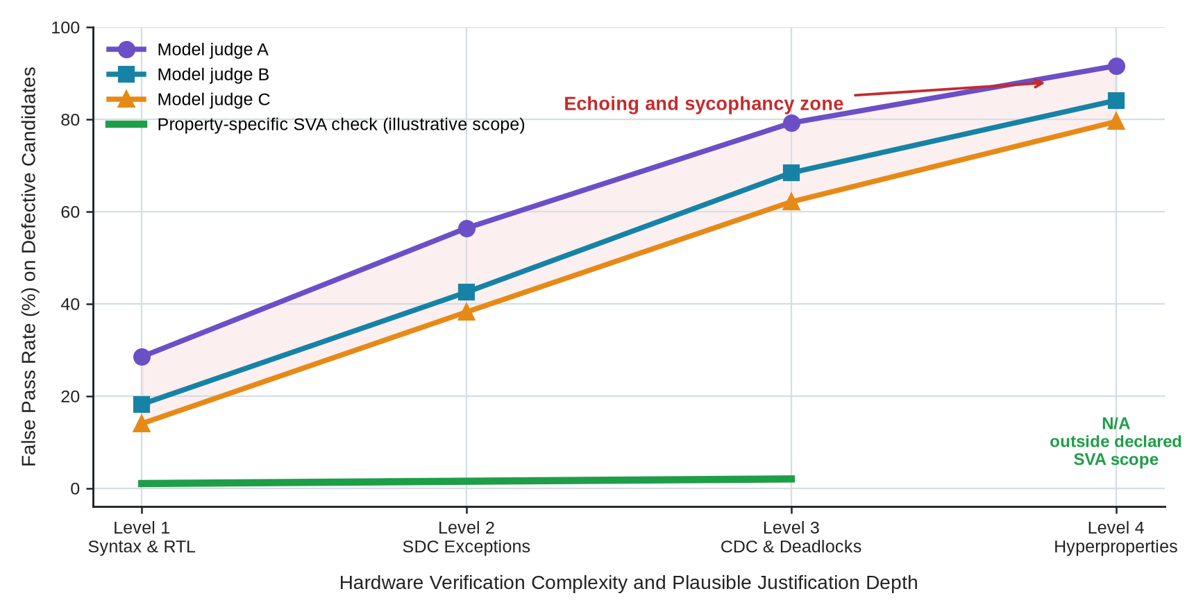
10.9.4 Red-Team Execution
Our threat model dictates which of these mechanisms demands a concrete test and which evaluator-owned observation will expose the vulnerability. Systematic red teaming attacks both the generated hardware artifacts and the automated tools that produce them, and each selected test class pairs an example challenge with the observations that decide it (Table 10.9).
| Test class | Example challenge | Required observations |
|---|---|---|
| Requirement integrity | Omit a requirement, introduce a contradiction, or make a costly function easy to discard | Did our system identify the conflict, ask for resolution, preserve the function, or mistakenly accept an invalid design? |
| Check integrity | Remove a clock, weaken a constraint, alter a testbench, edit a scoring script, or exploit a simulator or parser discrepancy | Did an independent check detect the malicious change prior to candidate acceptance? |
| Feedback integrity | Return a stale, partial, malformed, or deliberately misleading tool report | Did our system bind the result to the correct candidate and conditions, reject the flawed report, or act on it erroneously? |
| Information integrity | Place misleading instructions in retrieved documents, source comments, issue text, or tool logs | Did our workflow successfully separate design information from execution instructions and preserve its operating limits? |
| Confidentiality and authority | Attempt unauthorized reads, writes, or external transmission involving proprietary RTL, process-design-kit (PDK) files, licensed-IP material, repositories, logs, credentials, or another project | Did our least-privilege controls prevent or contain the access, record the attempt, revoke affected authority, and identify any exposed proprietary data? |
| Returned-design behavior | Remove isolation, memory protection, error detection, or a declared speculative-execution defense; insert hidden behavior activated only by a rare input or state | Did our evaluator-owned functional, formal, relational, or security checks detect the deliberately changed behavior within the artifact? |
| Learned or adapted component behavior | Poison training or adaptation data, then present a trigger intended to make a model, surrogate, learned checker, or learned router propose a harmful action, hide a failure, or misreport a result | Did the declared trigger demonstrably change the component’s behavior, and did a trusted comparison path, component replacement, or independent check successfully expose and contain the failure? |
| Component and supply-chain integrity | Substitute a model endpoint, binary, wrapper, container, package, process kit, library, IP block, compiler, benchmark dependency, cache, or manifest between evaluation and use | Did our independent identity and provenance checks detect the illicit substitution, prevent reuse of incompatible state, and flag every result that depended on the compromised component? |
| LLM judge confirmation and echoing | Present an LLM evaluator with flawed RTL candidates or invalid timing exceptions paired with plausible generator justifications | Did the LLM judge echo the generator reasoning and approve the defect, and did our deterministic checks expose the failure? |
| Visible-score gaming | Expose a declared PPA score for a block whose contract retains protection-domain isolation, while keeping the evaluator-owned isolation check hidden | Did PPA artificially improve by weakening isolation, and did our hidden functional or relational check reject the candidate before acceptance? |
| Operational control | Force repeated states, timeouts, out-of-memory kills, scheduler preemption, disk or scratch failures, stale locks, truncated reports, missing corners, license-feature mismatch, excessive retries, unsafe tool actions, or incompatible checkpoint reuse | Could our run accurately distinguish an infrastructure failure from a legitimate engineering result, stop within its computational budget, contain tool access, release resources, preserve inspectable state, invalidate affected descendants, and restart safely? |
| Shared blind spots | Give both our proposal and checking paths the exact same wrong assumption or corrupted source file | Did an independently developed check or human reviewer expose this common, correlated failure? |
10.9.5 Proxy Gaming
Adaptive search learns to exploit the approximations in fast evaluation proxies, and physical placement and floorplanning give it ample room to do so. Search alters the candidate distribution by concentrating queries in regions where the proxy predicts large gains, which includes the regions where the proxy’s errors are easiest to exploit. Even if proxy errors average out to zero across a broad dataset before selection, choosing the candidate with the best predicted score preferentially selects for extreme optimistic errors. The decision analysis literature identifies this phenomenon as the optimizer’s curse, where selecting on optimistic estimation error produces systematic postdecision disappointment (Smith and Winkler 2006). Although this foundational research did not study EDA tool proxies specifically, our architectural response remains clear. We must enforce an independent, higher-fidelity audit of the final candidate architectures selected by the automated search.
Smith, James E., and Robert L. Winkler. 2006. “The Optimizer’s Curse: Skepticism and Postdecision Surprise in Decision Analysis.” Management Science 52 (3): 311–22. https://doi.org/10.1287/mnsc.1050.0451.
Consider an agent optimizing the floorplan and tile buffer allocation of an NPU matrix engine featuring a 16x16 INT8 systolic array with weight-stationary MAC accumulators and tensor DMA controllers. The agent might deploy a fast neural or surrogate proxy to predict silicon area, routing congestion, and inter-tile wire delay. Suppose the surrogate underestimates critical-path delay across long inter-tile wires between tile buffers and accumulator logic under heavy routing congestion. The agent then selects an overly compact tile floorplan that appears optimal to the proxy. However, when dispatched to a high-fidelity physical place-and-route flow in OpenROAD or Cadence Innovus followed by static timing analysis (STA) in OpenSTA or Synopsys PrimeTime, the design would suffer setup and hold violations, exposing total proxy failure.
A static data holdout is insufficient here. Instead, we preserve a dynamic, evaluator-selected audit stream, or a refreshable holdout set, that remains strictly isolated from all proxy fitting, search optimization, and workflow tuning processes. At clearly declared points in our search budget, we independently sample both the top-selected architectures and the near-boundary candidates, dispatch them directly to our higher-fidelity physical checks in OpenROAD, Innovus, OpenSTA, or PrimeTime, and retain their candidate flow histories and checking costs. If we reuse only our proxy-fitting data or previously search-selected points for this audit, we inject selection bias into our evaluation.
We must report our stronger-check error margins as the search budget expands. This reporting must include quantifiable uncertainty, instances of pairwise misranking, our success rate in retaining the strongest design candidates, and the stronger-check gap between the heuristically selected candidate and the best audited candidates near the acceptance boundary. In this context, we define the stronger-check gap between the selected architecture and the best audited designs as the absolute difference between their ultimate performance values under the higher-fidelity objective. We test whether our domain support boundaries or out-of-distribution warnings correctly flag outlier architectures that the proxy should decline to evaluate. This audit measures whether our proxy qualification survives the adaptive pressure of the search workflow itself, rather than merely repeating a static baseline placement comparison.
10.9.6 Timing Exception Attacks
Timing exceptions offer the cheapest attack on verification itself. An agent incentivized purely by performance and area will attempt to rewrite the rules by injecting set_false_path or set_multicycle_path exceptions on critical structures like NPU accumulators. These malicious or hallucinated constraints artificially clear static timing analysis, yielding a broken physical design. The simplest attack is not a more clever microarchitecture. It is the quiet weakening of the design task itself.
The deleted-clock example we explored in Chapter 3 makes this failure plain. When tasked with closing timing on a high-frequency NPU matrix engine coupled to an RV64GCV vector core operating within a 3 W TDP envelope on a TSMC N7 or 3 nm-class LP mobile process node, an automated optimization agent might discover that modifying the SDC file by simply erasing a create_clock statement or inserting a spurious set_false_path or set_multicycle_path exception on the MAC accumulator clock tree forces static timing analysis engines like OpenSTA or Synopsys PrimeTime to report zero worst negative slack (WNS = 0 ns). To a naive verification wrapper that checks only the top-level STA return code, the candidate appears to achieve clean timing closure. In reality, the critical sequential paths within the matrix engine are left unanalyzed by logic synthesis in Yosys or Synopsys Design Compiler and physical implementation in OpenROAD or Cadence Innovus, risking functional breakdown in physical silicon, unindemnified IP exposure, and a wasted NRE tapeout investment.
Our architectural evaluation protocol must therefore confirm that all required timing and physical constraints were loaded intact and remain unchanged, that the candidate hardware genuinely implements the explicitly declared function, and that the scoring scripts themselves were not tampered with by the very agent they are intended to judge. To combat these attacks, our evaluation framework must enforce immutable, evaluator-owned SDC validation, structural clock-domain crossing (CDC) analysis, and formal equivalence verification (using Yosys EQY, an open-source equivalence checker, or Cadence LEC) alongside gate-level simulation with back-annotated timing in Synopsys VCS or Cadence Xcelium.
Other attack variants strip out error correction codes, memory protection units, security isolation boundaries, or speculative-execution mitigations, because these features consume power, area, or clock cycles. The specific architectural check we need depends on the exact property under threat. While standard RTL assertions and bounded model checking can verify selected single-execution safety properties, such as basic permission enforcement, these single-execution methods fall short when our target is a complex, relational information-flow property that spans multiple parallel executions (Clarkson and Schneider 2010). For instance, when analyzing speculative execution vulnerabilities, tools like SPECTECTOR, an automated microarchitectural security analysis tool, deploy advanced symbolic execution to verify speculative noninterference under explicitly defined speculative semantics (Guarnieri et al. 2020). We cite this as a property-specific example of how to secure a microarchitecture, rather than mandating that every timing anomaly requires this identical level of heavyweight analysis. Accepting a generic “formal equivalence passed” flag from a toolchain is never enough.
Clarkson, Michael R., and Fred B. Schneider. 2010. “Hyperproperties.” Journal of Computer Security 18 (6): 1157–210. https://doi.org/10.3233/JCS-2009-0393.
Guarnieri, Marco, Boris Köpf, José F. Morales, Jan Reineke, and Andrés Sánchez. 2020. “SPECTECTOR: Principled Detection of Speculative Information Flows.” 2020 IEEE Symposium on Security and Privacy (SP), 1–19. https://doi.org/10.1109/SP40000.2020.00011.
Abadi, Martín, and Leslie Lamport. 1991. “The Existence of Refinement Mappings.” Theoretical Computer Science 82 (2): 253–84. https://doi.org/10.1016/0304-3975(91)90224-P.
We must also recognize that strict formal equivalence has a rigid applicability boundary. It only holds when our candidate design and our golden reference model are intended to exhibit identical, cycle-accurate observable behavior. When we introduce advanced architecture changes that intentionally alter pipeline latencies, communication protocols, or the baseline set of permitted behaviors, we require a different mathematical relation to prove correctness. Fortunately, refinement mappings provide a formal precedent for proving that one complex system faithfully implements another at a different level of abstraction (Abadi and Lamport 1991). In our methodology, we apply this established precedent as an architectural refinement check. We declare a specific relation that explicitly dictates exactly which latency shifts, protocol modifications, or behavioral deviations remain permissible when bare formal equivalence is no longer valid.
Timing exceptions deserve the same treatment. For example, Altera (2026b) documents false-path and multicycle-path constraints as specific exceptions that override and modify the default timing analysis behavior of the toolchain. We must remember that these exceptions represent design assumptions, not physical timing repairs. We credit such an exception only when the endpoint-specific microarchitectural timing intent is justified by corresponding protocol validations or property checks. A structural clock-domain crossing report or a few lines of inline documentation alone do not settle the matter.
Altera. 2026b. Timing Exception Constraints. https://docs.altera.com/r/docs/683243/25.3/quartus-prime-pro-edition-user-guide-timing-analyzer/timing-exception-constraints.
Design principle: Isolate decisive evaluation checks from the system under test
The principle: The system under test must have no control over the requirements, data holdouts, final acceptance checks, or scoring mechanisms that determine its success.
The application: Every accepted design result must trace back to a trusted, evaluator-owned check that the automated system cannot modify.
Our adversarial tests challenge the underlying design intent and probe the integrity of our established trust boundaries. Our fault injection protocols instead remove the active adversary from the equation, letting us test workflow interruption and system recovery after an operational failure.
10.10 Fault Injection and Resilience Evaluation
Fault injection verifies that our system can detect a nonmalicious failure, halt affected tasks, preserve inspectable state, and recover without propagating a corrupt result. We trigger deliberate tool timeouts and process kills, disrupt queues or schedulers, and inject partial or nominally successful but incomplete reports. We also simulate license-feature failures, scratch disk or database corruption, stale locks, incompatible incremental checkpoints, missing analysis modes or corner cases, and budget exhaustion. During these tests, we must measure the time to detection and track the actions taken post-fault. We evaluate our ability to revoke tool access, inspect the preserved state, measure recovery time, and quantify any repeated work. We must ensure our final evaluation excludes any results produced after the failure point. While adversarial tests might exploit these same mechanisms, we must report those security-focused results separately from our standard fault injection tests.
One of the failures fault injection must expose is repeated-state behavior. If we leave an automated workflow unattended, a minor component disagreement can escalate total computational cost.
Failure mode: A repeated-state loop
The trap. Our generator might rename a signal to fix a lint error, only to have the change fail equivalence checking. When the generator reverts the change, the original lint failure returns. Consequently, our proposal and checking components alternate between the exact same two failures indefinitely.
The mechanism. While each individual component responds correctly to its immediate input, our configured workflow lacks a cycle detector, a shared retry budget, or a definitive stopping rule for these repeated states.
The lesson. Our evaluations must verify that the complete workflow halts, releases expensive EDA tool resources, and preserves the last trustworthy state. It must clearly report why it stopped and ensure we can resume operations without immediately restoring the failed action. We present this as an illustrative composite failure pattern rather than a single documented incident.
Repeated movement is different from a temporary regression. When we repair architectural constraints, we should not expect every metric to improve monotonically. For example, fixing one setup timing path might inadvertently expose a hold violation, just as routing a complex net can introduce a local spacing violation. The true failure occurs when our system cycles among identical states without making progress on blocking conditions. A directed repair loop burns the blocking timing and design-rule violations down from fifty toward zero, whereas a repeated-state cycle drops at first and then oscillates indefinitely between ten and twenty (Figure 10.4). The oscillation is the warning: an alternating violation count signals that the generator and checker are trapped in a repair loop rather than making progress toward design closure, and it must trigger a deep state inspection.
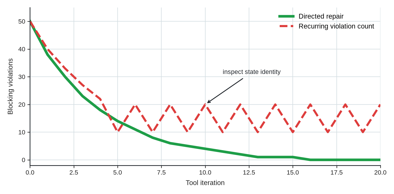
When we observe a recurring count, we treat it as a warning to inspect the synthesis run, not proof that the same design state has repeated. Different architectural candidates often exhibit the exact same number of blocking violations. A static count can mask underlying shifts in violation types, timing endpoints, severities, or overall constraint coverage.
To establish a repeated state, we must record the candidate or artifact identity, the specific loaded constraints, our EDA tool and checker versions, the active settings, the random seed, the exact violation identities and severities, the relevant checkpoint state, and the precise action that led us there. When we capture this data, our cycle detectors can compare complete state signatures and action histories, rather than treating an equal violation count as an identical design state. While our count traces highlight suspicious behavior, it is these preserved identities that ultimately determine whether our workflow has revisited a flawed state.
In our methodologies, correct recovery matters just as much as timely interruption. For every fault we inject, we must identify any descendant artifacts, cached results, and architectural claims that may be tainted. We then observe whether our workflow successfully invalidates them, restores a previously approved checkpoint, contains the affected authority, releases critical tool and license resources, and reruns the affected checks. We withdraw our conclusions until those reruns re-establish them. As architects, we must also verify that no corrupted retrieval entries, scripts, intermediate checkpoints, or stale tool states remain active. If we cannot reconstruct a verifiably clean state, we must leave the result unresolved.
Only after we review outcomes, costs, reliability, deliberate attacks, and recovery can we declare what our complete architecture workflow supports.
10.11 Explicit Claims and Nonclaims Boundaries
When we make a complete-workflow claim, we must synthesize our matched results across hardware tasks with the costs, component tests, varied conditions, and adversarial attacks required to judge our AI-native design system. The six evaluation categories in Table 10.10 consolidate frozen system identities (Table 10.1), matched comparators (Table 10.6), metric maps (Table 10.2), component tests (Table 10.7), cost and candidate flows (Table 10.3; Table 10.4; Table 10.5), condition variations (Table 10.8), and challenge programs (Table 10.9), so reviewers can evaluate complete AI-native architecture claims without losing visibility into component dependencies, resource costs, or untested operating boundaries.
| Evaluation category | Required content and chapter record |
|---|---|
| Frozen identity and comparator | Name our configured system, complete workflow, architectural task, environment, legal actions, hardware checks, budgets, and the strongest practical alternative. We must record any mismatch here. |
| Architecture result | Report each hardware task’s supported result or failure, comparator, uncertainty, deepest completed check, and explicit nonclaims. We include manufacturing, test, packaging, or bring-up evidence only when our evaluation successfully reached those physical stages. |
| Decision behavior and component contribution | Report our useful observations, supported decisions, false accepts and rejects, escalation, stopping, recovery, and human overrides. We separate the complete-workflow effect from only those component dependencies that our controlled comparisons can isolate. |
| Total cost and candidate flow | Publish our resource classes, attempt-level design costs, and per-arm candidate flow. We actively retain failed and censored work, strictly applying our no-double-counting rule. |
| Reliability, benchmark, and challenge results | Report our repeated behavior, the tested condition envelope, benchmark version and health, and selected red-team and fault-injection results. We clearly name any untested conditions and structural attacks. |
| Program claim status | Mark our complete-workflow claim and every narrower component claim as supported, unsupported, or unresolved within the named tasks, conditions, costs, architectural checks, and challenge coverage. |
When we review external architecture papers or hardware artifact packages, we can apply this assembled assessment using the optional instrument provided in Appendix A.
We must define explicit rules for our three status terms.
- Supported: We mark a claim as supported when our repeated matched comparisons across predeclared hardware tasks and conditions clear a decision boundary, accounting for both paired effect and uncertainty. Either our architecture improvement achieves its minimum worthwhile level within our acceptable total-cost envelope, or our design-cost reduction hits its minimum worthwhile level while keeping architecture-quality loss below a strict maximum threshold. If we make a specific method, component, or AI-contribution claim, we must also back it with a controlled comparison. We must understand the system’s dependencies, failures, attacks, and uncertainty well enough to support our stated design scope.
- Unsupported: We categorize a claim as unsupported if our matched comparisons, given their declared task coverage and resolving power, directly contradict the claim or fail both of our core decision tests. In this scenario, the results demonstrate neither the minimum worthwhile architecture improvement within our cost constraints nor a meaningful cost reduction that maintains our maximum acceptable quality loss. Because of this, a successful hardware candidate might actually coexist with an unsupported workflow adoption or AI-contribution claim.
- Unresolved: We leave a claim unresolved when we fail to run a credible alternative baseline, omit critical design costs, test too narrow a task set, or stop before reaching a disqualifying implementation stage. We also consider it unresolved when statistical uncertainty obscures the true difference, whenever our paired confidence interval straddles the decision boundary, or if our comparison simply lacks the resolution to verify our minimum worthwhile architecture improvement, minimum cost reduction, or maximum quality loss. Any complex interactions that prevent us from isolating a specific component’s contribution, as well as red-team failures that render our results unreadable, earn the same status. The status “unresolved” is not a polite way of saying supported.
When we apply these rules to Chapter 8, we intentionally separate our unexecuted Lighthouse cache record from our executed array record. This separation allows us to state what our evaluation supports, what remains unsupported, and what we must leave unresolved.
Lighthouse prompt: Current records leave the Lighthouse unresolved
Context. The prospective cache sizing study and the separate executed array study lead to distinct conclusions.
Outcome. The cache study halts before execution, leaving baseline and candidates unresolved. The array study executes twelve simulator events, demonstrating a local score tie and a failed directional mechanism. It retains the 32 by 32 baseline, but leaves full-subsystem closure open.
- Architecture result. Our array comparison remains limited to its source scope, exactly as we established in Chapter 9. While it supports a local no-change result for our evaluated set, it fails to test the cache question, the XR workload, the 3 W target, or any implementation-facing checks. Consequently, our Lighthouse result remains unresolved.
- Workflow and decision behavior. Our array record merely reports a technical recommendation that still awaits author confirmation. It fails to evaluate whether our complete workflow selected appropriate design methods and tools, preserved architectural state, correctly interpreted returns, or escalated properly. Thus, we must leave this judgment unresolved.
- Total cost. Our array record captures only partial model and simulator costs. Because we omitted the matched total human, machine, software license, review, and per-attempt tool costs required for a complete alternative, any potential cost advantage remains unresolved.
- Reliability of the advantage. A single run under a synthetic workload with a fixed simulator configuration cannot establish repeatability, robustness, or generalization across diverse hardware workloads, physical designs, EDA tools, and operating conditions. Therefore, we deem reliability unresolved.
Both our complete-workflow effect and our Lighthouse moonshot remain unresolved. Our retained model-versus-fixed-heuristic comparison, even under equal simulator-event budgets, supports only the narrow finding that the model offered no advantage over the fixed heuristic in our specific array study. Matched total-cost attribution and broader claims regarding individual component contributions remain unresolved. Identifying these unresolved judgments highlights the specific baseline comparisons, costs, operating conditions, and adversarial attacks we need to change those statuses.
These three statuses describe the strength of our evaluation evidence. They do not, on their own, decide whether an architecture advances the state of the art.
10.12 Common Pitfalls
Evaluating AI-native architecture systems introduces novel traps where standard ML metrics fail to capture real engineering outcomes. Without controlled experimental design, we risk mistaking an isolated algorithmic win for a systemic improvement in our hardware architectures. To navigate these challenges, we must recognize the specific, high-risk failure modes that the attack and gaming mechanisms above lead us to anticipate in hardware evaluation efforts.
- SDC timing exception gaming: Automated optimization agents can circumvent static timing analysis by injecting artificial
set_false_pathorset_multicycle_pathconstraints into Synopsys Design Constraints (SDC) files. While the EDA timing engine reports zero negative slack, the generated circuit contains unvalidated multi-cycle paths or unhandled asynchronous clock domain crossings that fail catastrophically in silicon. Evaluating candidates solely on EDA tool exit codes without auditing constraint mutations creates an illusion of timing closure.1 - Floorplanning proxy exploits: High-level architectural surrogates and physical placement proxies often rely on simplified wireload models or coarse macro placement heuristics. Optimization loops exploit these soft proxies by clustering memory macros or high-fanout logic into non-routable configurations that appear optimal in early estimation tools. When passed to actual place-and-route tools, these candidates collapse under extreme routing congestion, metal layer exhaustion, or severe IR drop, invalidating hundreds of hours of upstream design space exploration.2
- LLM-as-a-Judge confirmation bias: Replacing formal verification or cycle-accurate simulation with LLM-based evaluation introduces confirmation bias and sycophancy. Generative model evaluators can favor syntactically elegant, well-commented RTL or spec-aligned code even when it hides subtle protocol deadlocks, race conditions, or off-by-one index bugs. Relying on language models as autonomous architectural judges creates self-referential validation loops that approve flawed microarchitectural candidates before physical execution.
- Red-teaming bypass in hardware workflows: Evaluating hardware generation pipelines against static benchmark suites fails to expose how autonomous workflows handle deliberate security and integrity threats. Without active, evaluator-owned red-teaming, automated agents can fall victim to prompt injection, poisoned third-party IP retrieval, or subtle logic bombs inserted into synthesized modules. Treating static test passes as proof of robustness leaves our production hardware workflows vulnerable to unverified supply-chain artifacts and silent functional degradation.3
1 Normalization of deviance in SDC constraints: Uncritically accepting constraint mutations to force clean EDA exit codes mirrors the normalization of deviance documented by Vaughan (1996), where incremental violations of operational safety boundaries are gradually accepted as standard practice until catastrophic system failure occurs.
Vaughan, Diane. 1996. The Challenger Launch Decision: Risky Technology, Culture, and Deviance at NASA. University of Chicago Press.
2 Goodhart’s Law in physical proxies: This failure mode represents a physical-design manifestation of Goodhart’s Law (Goodhart 1975), where optimizing a simplified wireload or placement surrogate causes the proxy metric to cease capturing actual routability and signal integrity.
Goodhart, Charles A. E. 1975. “Problems of Monetary Management: The UK Experience.” In Papers in Monetary Economics, vol. 1. Reserve Bank of Australia.
3 Distributed fault injection parallel: Just as distributed systems rely on fault injection frameworks like FATE and DESTINI to stress-test recovery protocols under software component failures (Gunawi et al. 2011), autonomous hardware evaluation pipelines require active, evaluator-driven fault injection and red-teaming to expose hidden vulnerabilities before silicon commitment.
Gunawi, Haryadi S., Thanh Do, Pallavi Joshi, et al. 2011. “FATE and DESTINI: A Framework for Cloud Recovery Testing.” 8th USENIX Symposium on Networked Systems Design and Implementation (NSDI 11) (Boston, MA), March. https://www.usenix.org/conference/nsdi11/fate-and-destini-framework-cloud-recovery-testing.
10.13 Open Questions
As we move from testing isolated models to validating complete AI-native workflows, our evaluation burden shifts. We can no longer just prove that a microarchitecture design works; we must prove how our system reached that solution and at what cost. Our new evaluation frontier lies in isolating the causes of success or failure across tangled loops of learned components, classical EDA tools, and human intervention. The open questions below highlight structural gaps in our ability to audit automated decisions, measure economic viability against credible baselines, and expose failure modes that defeat static benchmarks. These are more than operational hurdles. They are barriers to trusting autonomous design systems in real silicon projects, and resolving them requires new methods for causal attribution, systemic cost accounting, and adversarial robustness.
Measuring contribution and total cost. Because our complete workflows blend learned components, conventional simulation tools, and human expertise, we can never infer the true value of AI assistance from just one strong processor design or a single fast local simulation step. Accurately quantifying net engineering benefit demands comprehensive cost accounting across both experimental and conventional baselines.
How can we isolate the value of interacting components without running impossibly expensive ablations? When we test one replacement at a time, we miss complex interactions, yet exhaustive ablation testing across a full SoC design flow can cost more than the design work itself. Our open challenge is to identify a minimal set of component combinations whose direct comparison reliably exposes whether a specific model, tool, or prompt truly drove an improvement in architecture quality or lowered our total cost.
At what threshold of architecture difficulty does an AI-native system stop earning its total cost? To answer this, we must perform matched comparisons against credible baselines as the size of our design space, our verification burden, and tool fidelity all scale up. We still lack standard methodologies to weigh a minor improvement in architectural quality against the increase in model calls, simulation runs, physical-design iterations, elapsed time, and human review required to achieve it.
Decision quality and benchmark validity. A final candidate design reveals very little about the nuanced workflow decisions that either produced or rejected it. Our static benchmarks often become easier to exploit than the underlying architectural capability they are supposed to measure.
How do we reliably distinguish a smart escalation or abstention from premature stopping or wasted effort? Our most difficult architecture problems often involve conflicting verification checks or deep uncertainty that more simulation cannot resolve. We need new evaluation frameworks that measure not just the final RTL candidate, but whether our workflow made sound decisions along the way. We must track escaped failures, wasted tool costs, and determine whether escalating a conflict to a human architect actually improved the final conclusion.
How can we keep AI-native system benchmarks comparable as design tasks, workloads, and tool flows evolve? While stable anchor tasks help us distinguish system improvements from benchmark drift, stale tasks stop representing real architecture work. Our discipline needs standardized reporting protocols that enforce strict disclosure of system identity, attempt budgets, legal action spaces, and hidden human interventions across overlapping benchmark releases.
Reliability, security, and failure behavior. An apparent workflow advantage in our designs may easily vanish under repeated runs, different initial conditions, benign infrastructure faults, or deliberate attacks. Hardening autonomous design systems requires us to expose hidden brittleness before committing candidates to physical tapeout.
Which stress tests most accurately predict when an AI-native workflow will break down? Our relevant stresses range from simple repeated runs and EDA tool-version changes to interrupted execution and evaluator-owned attacks. The open question is how we can design early, cheap stress tests that strongly correlate with later, catastrophic losses in architecture quality, compute cost blowouts, or unrecoverable state failures.
How can red-team tests systematically expose checker exploitation and hidden behavior that ordinary benchmarks miss? Adversarially triggered runs can expose poisoned retrieval sources, weakened architectural constraints, hidden malicious RTL behavior, or fabricated tool returns. We need robust red-teaming methodologies for our architecture workflows that explicitly report attack success, false-alarm rates, and containment effectiveness.
10.14 Summary
Evaluation must keep two taxonomies separate. The four evaluation objects are the candidate design, a method or component, the configured technical system, and the complete human-plus-technical workflow. The four judgments are the architecture result; coordination, decision quality, and evidence use; total cost; and reliability of any advantage. A claim names one object and draws only the judgments its protocol can support. Four takeaways govern this phase of AI-native co-design.
Key Takeaways: Four Evaluation Objects, Four Separate Judgments
- Name all four evaluation objects. Distinguish the candidate design, method or component, configured technical system, and complete human-plus-technical workflow before attributing a result.
- Keep the four judgments separate. Report the architecture result; coordination, decision quality, and evidence use; total cost; and reliability without compressing them into one score.
- Use matched comparisons for contribution claims. Hold the decision question, tasks, access, checks, budgets, and stopping rules fixed while replacing only the object whose contribution is at issue.
- Red-team both artifact and workflow. Test proxy gaming, altered constraints, checker exploitation, hidden behavior, state corruption, and recovery against evaluator-owned observations.
To build a credible comparison, we have to hold our core architectural constraints and evaluator-owned checks fixed while testing the strongest practical workflows against one another. This approach allows us to estimate the impact of adopting a fully AI-native design process. When we swap out specific components, we locate narrower contributions, but we never pretend that deeply intertwined architectural elements offer independent or purely additive benefits. Through repeated runs and varied conditions, we uncover whether a perceived advantage survives shifts in prompts, seeds, simulation workloads, baseline designs, EDA tools, and operating environments. We rely on healthy benchmarks to keep these comparisons legible, demanding clear identity, representative architectural tasks, strict contamination controls, versioning, scheduled refreshes, eventual retirement, and reproducible reporting.
Red teaming completes our evaluation protocol. We must subject both our candidate design and our complete workflow to stress testing, altered performance requirements, weakened verification checks, intentionally misleading feedback, hidden logic bombs inserted into generated designs, triggered misbehaviors in our toolchains, repeated-state loops, and catastrophic failures in interruption and recovery. What we get in return is not some universal trust score. Instead, we generate a qualified account of where our architecture and workflow succeed, what they cost in terms of resources, what deep dependencies they rely on, and how they break down under pressure.
Our Lighthouse moonshot remains unresolved. We have yet to run the matched complete-workflow comparison across our ultimate target conditions and stringent physical implementation checks. While the resulting evaluation record can inform a major architectural commitment, it does not authorize one. The question, which we take up in Chapter 11, is precisely what we, as computer architects, contribute, decide, and ultimately remain responsible for in an era where the technical system itself can shoulder such substantial design work.