9 Pattern Transferability and Generalization

“There is no single development, in either technology or in management technique, that by itself promises even one order-of-magnitude improvement in productivity, in reliability, in simplicity.”
— Fred Brooks, No Silver Bullet (1987) (Brooks 1987)
Author’s Note. Fred Brooks warned against expecting any single technique to remove the essential difficulty of software engineering. The transfer of these concepts to computer architecture is our synthesis, rather than Brooks’s original claim. When we port an architectural result to a new design problem, the underlying study structure may successfully transfer. However, our evidence remains tied to the original conditions under which we produced it, meaning we cannot assume conclusions automatically hold in a changed environment.
North-Star question
We rarely begin architectural design with an empty repository. Whether targeting CPU ISA extensions (such as RISC-V Vector / RVV 1.0, an open vector instruction set architecture extension, or ARM Scalable Vector Extension 2 / SVE2, an open SIMD instruction set architecture extension), NPU tensor dataflows, Triton (an open-source domain-specific JIT compiler framework), or a changed semiconductor process, current challenges often resemble completed projects. While leveraging prior work saves effort, it risks carrying forward obsolete assumptions or stale configurations that fail to support new decisions. We must determine exactly which components transfer safely, what context shifted, and which validation checks we must now execute. The rise of AI-native co-design makes this scrutiny urgent, as training data, learned heuristics, wrappers, and generated hardware artifacts remain viable for vastly different lifespans.
As we examine how prior work transfers across the design stack, we find it operates at three distinct levels, each carrying its own verification burden. Our core principles and experimental procedures transfer broadly because they structure how we study a new architectural decision. Conversely, our hardware and software components transfer only as long as their dependencies and target validation checks continue to support them. Our final conclusions, however, stand apart. They demand fresh target evidence the moment our design problem shifts. A durable architectural pattern gives us a robust methodology for reopening a claim; it is never a promise that our earlier answers remain correct under new constraints. Provided our decision parameters and acceptance semantics remain fixed, we only need to reopen those claims that depend directly on a material change in the system. Throughout this chapter, we refer to this tightly scoped reopening process as selective requalification. We operationalize this principle through a structured five-stage transfer test.
Learning objectives
This chapter establishes the following learning objectives:
- Identify when a target change reopens prior architecture claims or creates a new design problem.
- Partition source systems into discrete transfer units, map dependencies, and assign target actions.
- Translate changed conditions into concrete target tests or explicit untested boundaries.
- Evaluate complete system costs by charging interface overhead, offload granularity, and executable software paths against local results.
- Prevent stale reuse by scoping conclusions to their artifact versions, workloads, and evaluated conditions.
9.1 Evaluating Pattern Transferability and Scope
Evaluating transferability forces us to ask whether a new target still poses the identical architectural decision as our source system. Before allowing any prior conclusion to carry forward, we must decouple reusable structural units and their design actions from the target checks required to validate them under changed constraints. Our transfer framework traces how system shifts disrupt specific architectural dependencies through five progressive stages, ranging from initial decision comparison to target evidence enforcement. Rather than executing these stages as a rigid script, we use them to isolate exactly where source assumptions break down.
In any complex system, our source record mixes reusable components with an architectural conclusion whose validity is tied to the original problem. The transfer test moves source artifacts through its five stages and splits them along the way into two pathways: one that isolates the historical conclusion, one that carries the reusable components (Figure 9.1). That separation is the chapter’s central claim: reusable structural components may transfer under valid target checks, but their historical conclusions stay isolated and cannot by themselves validate a new design decision.
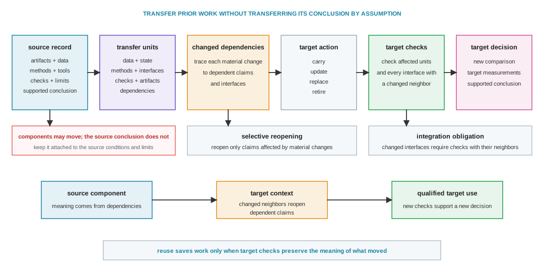
As we trace this workflow, the top path prevents a reusable simulator, performance predictor, interface, or hardware artifact from implicitly carrying over an architectural conclusion that our target environment has not actually established. Conversely, the lower path defines exactly what makes our reuse defensible. We recognize that a source component remains valuable only when we can identify its dependencies, and when our target checks cover both the affected architectural claims and any changed system interfaces.
Successful transfer allows us to move useful engineering work without blindly moving the original source conclusion. We define the complete configured technical system as our versioned composition of data, represented state, design methods, interfaces, tooling, validation checks, and configurations. While people, organizational capacity, hardware access, and decision authority remain necessary operating conditions for our design cycles, they sit structurally outside this core technical object. A definitive transfer result tells us exactly what prior architectural work still supports our new target; however, it does not by itself prove that introducing an AI-native methodology into our workflow is worthwhile.
Design principle: Transfer components, not conclusions
The application: Prior architectural conclusions must never be transferred without executing fresh target checks.
As we apply this framework, our initial decision comparison serves as our admission check, determining whether the new target truly retains the original source decision semantics. The remaining stages force us to systematically trace which dependencies changed, along with the specific architectural claims and interfaces those changes disrupt. Because permitted design actions, system observations, optimization objectives, failure classes, feedback loops, and commitment rules often vary across different architecture problems, our procedure preserves these nuanced differences rather than forcing every design into a single, rigid tool sequence.
9.2 Target System Shifts and Decision Reopening
When our initial decision comparison reveals a target system shift, it reopens prior architectural decisions whenever new workloads, silicon constraints, or interface contracts break the assumptions behind the original problem formulation. We define a design problem as the complete decision context that gives alternatives their meaning. It explicitly names the decision we must make, along with the candidate, artifact, or system boundary to which that decision applies. We use it to define our workload, software stack, implementation details, and system conditions. A well-formed design problem states exactly what we can and cannot change, identifies our constraints and credible architectural comparators, specifies the required measurements and checks, and accounts for the cost and reversibility of a wrong choice.
We must therefore distinguish a design problem from a benchmark, a candidate, a method, or a simple tool invocation. While a benchmark supplies our workloads or tasks, it does not dictate what aspects of the system we are allowed to modify. A candidate simply represents one architectural alternative within the broader problem. A method might propose, estimate, or select work inside that space, and a tool invocation merely observes a specific property under controlled conditions. None of these elements carries the full decision context on its own.
When we set up our target comparison, it serves two primary functions. First, it determines how broadly we need to recheck our prior claims. Second, it identifies exactly what kind of underlying change broke the support for those claims.
How broadly prior claims must be rechecked. We can apply selective requalification only as long as our target decision and acceptance semantics remain in force. If a material change occurs, we must reopen the specific architectural claims that depend on it.
What kind of change occurred. These changes typically take one or more of the following forms.
- Distributional transfer. Our objective, legal actions, artifact boundary, and acceptable-result definitions remain stable, but we shift the workload, operating conditions, or candidate population within that defined space (for example, shifting batch sizes or input frame rates while keeping the established CPU ISA extension principles or Triton compiler IR constant).
- Component or integration transfer. Our core decision remains stable, but we introduce a difference between the source and target in a component, interface, tool, library, or process condition along the executable or measurement path (for example, advancing Triton JIT compiler lowering and LLVM, an open-source modular compiler infrastructure, target generation principles, switching established CPU ISA extension principles such as ARM SVE2 to Advanced Matrix Extensions, Intel AMX, or altering NPU tensor dataflows).
- New design problem. We fundamentally change the meaning of our objective, legal actions, artifact boundary, or acceptance criteria (for example, transitioning from unconstrained datacenter throughput to a strict 3 W mobile headset power envelope).
We must apply these distinctions to each individual claim and dependency, rather than applying them uniformly across the entire target. A single target change often combines these forms because it breaks multiple, distinct dependencies in our architecture. We might use selective requalification for claims affected by a distributional or component change, but a new design problem forces us to reopen every claim tied to those modified decision semantics. The raw size of a change does not dictate our response. A large workload shift might still fall under the same design problem, whereas a seemingly trivial one-line tweak to our objective or action space can spawn a new one.
We consider a change to be material to a claim when it alters the candidate identity, executable path, measured quantity, objective, decision rule, ranking, constraint verdict, or the underlying mechanism on which that claim relies. Materiality is claim-specific. If we update our compiler toolchain, we might need to reopen our executable performance claims without touching our RTL functional properties. Similarly, if we shift our library or operating-corner, we reopen our timing and power analysis without necessarily invalidating our compiler-semantics results.
Every component and comparison we build carries a support region (the joint set of workload, design-family, tool, library, process, interface, and version conditions under which we originally qualified it). A source-to-target shift emerges whenever we propose taking work qualified in one region and applying it to another. Our discussion in Chapter 7 introduced distribution shift for changed data-generating conditions (Quiñonero-Candela et al. 2009) and a drift signal to track observed changes over time. However, we also face material changes in our software stacks, tools, libraries, process calibrations, or hardware interfaces. These architecture-specific changes extend far beyond standard model-distribution drift; our executable or measurement paths can shift even if a model’s input distribution remains stable. When this happens, we feed the affected claims back through our standard classification process rather than inventing a new category.
Standard dataset-shift tests compare a reference sample against incoming data and report when those distributions diverge (Rabanser et al. 2019). In our discipline, we must reopen the affected support claim the moment we detect such a shift. The shift signal itself does not identify the root cause, prove that our architecture decision has been compromised, or grant us permission to blindly reuse, recalibrate, adapt, or retrain. To take those actions, we must execute the dependency analysis and target checks we develop throughout this chapter.
To ground this transfer framework, we turn to our preliminary spatial array experiment from Chapter 8. The retained source record includes raw simulator outputs, candidate definitions, configurations, software-stack identities, and local evaluation metrics. It does not include per-evaluation commands and logs, an exact prompt identity, a repository-commit binding, or an independent validation receipt. Those gaps rule out independent replay and strong causal attribution, but the retained outputs still support the narrow local comparison established in Chapter 8. Evaluating five spatial-array shapes in SCALE-Sim, a cycle-accurate systolic-array simulator (Raj et al. 2025), on a synthetic three-layer matrix multiplication slice, the study recommended retaining a 32 by 32 array based on a local score ratio of simulated cycles to average utilization. Its ranking and recommendation remain confined to that source context.
Our changed target now asks whether a 32 by 32 systolic-array shape (featuring 32 rows and 32 columns of processing elements), together with its compiler-visible tiling and memory-interface contract, should be frozen for RTL implementation in our Lighthouse spatial-tracking subsystem. Because we expanded our scope to encompass software and implementation contracts, our necessary checks now include functional correctness, timing closure, power envelopes, and electrothermal behavior. Our core transfer problem is to determine which pieces of our source work can accelerate this new target effort without mistaking a high-level simulator result for a final implementation decision.
While our implementation-facing target is deliberately narrower than the complete XR system, we cannot treat it merely as the next stage of our original source claim. It fundamentally alters our artifact boundary, our set of legal choices, our acceptance criteria, and our consequences of error. Consequently, we must treat this case as a new design problem rather than a simple selective requalification of our executed array study.
To frame our new target question, we explicitly name the artifact, the interface contract, and the critical commitment at stake.
Should the 32 by 32 reference, together with its compiler-visible tiling and memory-interface contract, be frozen for RTL implementation in the Lighthouse subsystem?
At this stage, our legal target candidate set and credible architecture comparator remain undeclared. Since our source study’s five shapes and locally retained 32 by 32 reference fail to define either element for our new design problem, we cannot run the target comparison yet.
Our target carries all eight layers of the Lighthouse prompt stack as required scope, incorporating XRBench alongside SPEC CPU2017 and MLPerf Mobile. The intended hardware and toolchain span an RV64GCV processor, an NPU spatial tensor accelerator, UCIe or CXL interfaces where the product boundary requires them, memory-system models, compiler lowering through Triton, MLIR, and LLVM, physical implementation, power intent, formal checks, and electrothermal analysis under a 3 W TDP envelope. These are obligations of the target study, not fixed experimental conditions. We have not yet selected a process design kit, standard-cell or memory libraries, process node, process-voltage-temperature corners, executable tool path, or licensed access arrangement. Referring to TSMC N7 and 3 nm-class processes as alternatives therefore defines an unresolved target boundary rather than a single implementation setup.
We cannot simply read the final answer directly from our source record. Freezing an interface propagates effects throughout the system. It dictates compiler behavior, SRAM organization, interconnect traffic patterns, host synchronization, physical power delivery, and even future software capabilities. Each of these effects introduces an additional architectural obligation rather than replacing an earlier one. While every source result retains its local meaning, we must reassess every source check before applying it to our new target, because our source and target share artifacts without sharing a complete decision context. As architects, we can inspect the simulator outputs, workload records, candidate definitions, and tool configurations independently from the represented project state, our proposing and checking methods, tool interfaces, the runtime environment, and our final conclusions. This separation matters because neighboring architectural components often demand different transfer decisions. For instance, we might find that a simulator wrapper remains functionally correct even after its underlying calibration expires, or that a predictor retains a useful structure long after the specific decision it previously supported ceases to apply.
9.3 Decoupling Transfer Units Across System Boundaries
To navigate these differing component lifetimes, we make source-to-target comparisons actionable by precisely naming and decoupling our transferred units. Data, state, methods, tools, checks, and conclusions rarely share a single lifetime in any architecture project. Treating them as an indivisible package forces an unhelpful choice between copying everything blindly or rebuilding the infrastructure entirely. Decoupling these elements establishes a foundation for identifying dependencies and validating transfer conditions.
9.3.1 Mapping Dependencies
Every transfer unit we define carries an invariant (a core relation that must remain true across both source and target for the unit to retain its meaning). An invariant is much more than an unchanged file. It might represent the functional behavior preserved by a module interface, the precise units and meaning of a performance measurement, the correspondence between a formal model and our RTL artifact, or the comparator we use to interpret an evaluation score. A unit’s dependencies simply name whatever might break that critical relation.
We should scope our transfer units to the smallest versioned boundary that possesses a declared interface or invariant, provided we can still apply an independently meaningful target check. If we cannot isolate a dependency with such a check, we must include it in the same unit. For example, when we compile a Triton kernel module or an LLVM IR representation (LLVM being an open-source modular compiler infrastructure) targeting CPU ISA extensions (such as RISC-V Vector / RVV or x86 AVX-512), we can only treat the compiler toolchain version (e.g., Triton 2.1 vs 3.0, or LLVM 18 vs 19) and the generated binary as separate units if we fix their identities and inputs, and when we can qualify the binary independently using a semantic-equivalence or application binary interface check. Otherwise, we have to transfer and check the entire compiler-to-binary lowering path together.
The transfer map puts Steps 2 through 5 of the test, from unit separation through target evidence checking, into practice. For each kind of transfer unit, it names the action a broken dependency permits and the target check that action then requires (Table 9.1). The discipline is the same down every row. A single target shift demands tailored, unit-specific actions rather than one uniform reuse policy, and each action pairs with a domain-specific check on held-out tasks or hardware references, so a reused artifact never carries a stale conclusion into its new context. For learned components, held-out means target tasks kept apart from any fitting or calibration.
| Transfer unit | Changed dependency | Valid action | Required target check |
|---|---|---|---|
| Data, records, and current knowledge | Workload, design space, objectives, provenance, collection conditions, specifications, manuals, libraries, or project documents differ. | Reuse the historical record; refresh target data and sources; retire stale sources; narrow unsupported coverage. | Check trace and artifact provenance, source identity and version, target coverage and exclusions, source-to-target overlap, and whether retrieved material supports the target fact. |
| Representation and project state | Constraints, interfaces, artifact versions, or cross-layer relationships differ. | Refresh live state; adapt the representation; replace a representation that hides a required relationship. | Check schema and constraint completeness, version consistency, and integration with neighboring state. |
| Learned component | Training support, inputs, outputs, objectives, constraints, project facts, or data-generating conditions changed. | Requalify the unchanged component; rerun a generator or optimizer; recalibrate a numerical mapping; adapt, retrain, replace, or retire the component when needed. | Test every role it fills on held-out target tasks, including accuracy or calibration, candidate legality, objective quality, stale knowledge, failure classes, and performance against the declared comparator. |
| Conventional method | Analytical assumptions, solver formulation, design space, or objective changed. | Reuse, adapt, rerun, replace, or retire the method. | Check its assumptions on the target and compare its target result with the same decision rule used for other methods. |
| Tool interface and environment component | Command syntax, parameter meaning, output schema, status codes, tool or library version, constraint and configuration files, random seed, license, runtime, machine resource, reset behavior, or isolation changed. | Refresh configuration; adapt, replace, or retire the component; rerun affected work. | Check target-version execution, interface parsing and failure classification, constraints and stochastic state, reset and isolation behavior, resource accounting, and integration with connected tools. |
| Empirical screening check | Target coverage, observed conditions, error tolerance, or relationship to the target reference changed. | Requalify before reuse; recalibrate only when a numerical mapping or threshold changes; adapt, rerun, replace, or retire the check. | Measure target support and class-specific errors against a separate reference capable of observing the property at risk. |
| Formal, equivalence, deterministic, or rule-based check | The target specification, assumptions, properties, representation relation, rules, or tool version changed. | Review the specification mapping; requalify the target setup; adapt, rerun, replace, or retire the check. | Check property and assumption coverage, the relation being established, target tool integration, and known positive, negative, and inconclusive cases. |
| Routing or escalation policy | Check cost, consequence, qualified coverage, or available review capacity changed. | Adapt, replace, narrow, or retire the policy. | Exercise routing thresholds, uncertain cases, failure injection, escalation, and resource limits on the target. |
| Configured system | Any neighboring component or interface changed, even when this configuration did not. | Rerun target integration; recompose, adapt, replace, narrow, or reject the configuration when required. | Repeat the end-to-end target task with pinned versions, total product-path costs, failures, and a credible alternative. |
| Architecture and AI-contribution conclusions | The target decision, comparator, budget, or measured path differs from the source. | Narrow the conclusion to its supported source scope or reject its transfer. | Repeat the architecture comparison and the matched AI-contribution comparison under target conditions. |
We often find that a single target change demands different actions across our data, methods, executable environments, checks, and configured systems. We must treat our final architecture and AI-contribution conclusions differently from the raw components. A conclusion is never just a component we can update mechanically; we must either narrow it to the conditions we have already tested, or reject it for our new design decision.
When we select an action, it must match our target need, and we use each of these terms under a formal requalification contract. A requalification contract specifies the exact broken dependencies, invariant checks, minimal target test sets, and acceptance criteria required to re-verify an existing component or claim before it can be safely accepted under a new design context. Each action (whether we reuse an unchanged unit, refresh live data, requalify via contract, recalibrate thresholds, adapt an interface, retrain a learned model, recompose a configuration, replace a component, or retire obsolete work) defines a specific architectural transformation. Rejecting a component’s target use never erases the valuable historical source record; it simply prevents stale evidence from polluting the new decision context.
While machine-learning literature defines negative transfer as a transferred or adapted method performing worse on the target than a target-only alternative (Zirui Wang et al. 2019), we must extend that concept. In our synthesis, we elevate that comparison from simple model performance to overall architecture decision quality and total methodology cost. Whenever our studies claim that a transferred or adapted component provides a concrete transfer benefit, we must run a matched target-only comparison. In this setup, we provide both arms with the identical target problem, tasks, target-data availability, tool access, compute budgets, review capacity, and stopping rules. We give the target-only arm no source unit under test, and we explicitly disclose any conventional infrastructure shared by both arms. We also ensure our total cost accounting includes adaptation, requalification, integration, and eventual retirement or recovery, alongside the baseline costs of use and checking. Other affected units still require their own target checks; however, we do not need a matched with-and-without comparison for every reused historical record, tool interface, or deterministic artifact. If we discover a harmful prior, we must retire it immediately. If a prior proves merely cost-neutral, it cannot support a claim of transfer benefit; we should only keep it if it improves another declared target criterion once all use and checking costs are fully counted.
9.3.2 Isolating Design Slices
Our dependency columns do more than list inputs; they actively identify the affected slice of our configured system. For instance, when we update a compiler toolchain (such as changing an LLVM vectorization pass or a Triton JIT lowering version), we reopen our generated code, runtime behavior, and performance measurements, but we do not need to reopen an unrelated RTL equivalence result. Similarly, a process-library update or NPU tensor dataflow shift (such as moving from weight-stationary to output-stationary tile scheduling) forces us to re-evaluate timing, memory power, and any predictors trained on the old dataflow layout, even though it preserves our compiler-level language semantics perfectly. When we use our map, we limit our requalification efforts to the claims that rely on a broken invariant. We then add a targeted integration check wherever our affected component meets an unchanged neighbor.
We must be precise in our terminology. Only learned components can be retrained. We can refresh data, adapt representations, replace tool interfaces, or recalibrate checks, but none of these actions constitute retraining unless the unit itself learns directly from data. Consider, for example, a congestion predictor trained on prior routed designs. We treat its learned weights and feature schema as the transferable artifact, while our target inputs consist of placed netlists alongside the selected process and library features. Before we reuse this predictor, our target checks must establish that the new netlists satisfy the predictor’s input schema and fall within our legal target design family. We must recalibrate our thresholds when necessary, and compare class-specific errors and calibration against held-out routed target designs. The predictor’s weights do not carry our live project state, our current routed results, or our final architecture conclusions; we must generate and track those as explicit target artifacts.
To isolate affected design slices, we diagnose broken invariants across five system failure modes, covering workload-support mismatches, candidate-family shifts, proxy-reference correlation loss, executable-path disruptions, and decision-semantics changes. While Table 9.1 formalizes the specific transfer actions and required checks for each architectural unit, our diagnosis focuses on identifying the root invariant behind each broken dependency. A workload shift or expanded candidate population requires validating model coverage against target distributions; a changed process node or memory library demands fresh proxy-to-reference calibration; toolchain updates require compiler-generated integration checks; and altered objective criteria signal a brand-new design problem rather than simple component reuse.
When examining machine-learning studies on distribution shift and hidden dependencies alongside our negative-transfer test, we extract three lessons that we must make concrete for computer architecture. First, our empirical support can expire even when a component’s interface remains unchanged. Second, our local metrics can easily blind us to a broader system failure. Third, our attempts at adaptation can actually perform worse than a clean, target-only alternative (Zirui Wang et al. 2019; Quiñonero-Candela et al. 2009; Sculley et al. 2015). In our architectural methodology, we must recognize that these relevant conditions span not just workloads and candidate families, but also our specific compiler, tool, library, process, interface, and hardware versions.
These lessons force us to cleanly separate four terms we too often conflate. Generalization asks whether our component performs reliably on unseen cases that still fall within our declared target support. Transfer asks whether our source unit remains useful after our target environment changes materially. Robustness asks how our system’s behavior changes when subjected to named perturbations, faults, or attacks. Drift describes an observed, temporal change in a monitored condition or distribution. We must gather separate, specific evidence for each of these phenomena. Our ultimate architectural conclusion rests on whether our fully configured system supports our target decision under its named conditions. We might find that a predictor retains high accuracy even as our executable path or decision rule shifts, just as a correct tool wrapper might remain locally valid while a change in its neighboring configuration renders the complete system result unusable.
At the component level, an unchanged component that passes the relevant target checks may carry forward within the checked scope. An adapted component requires a new target evaluation. A change in decision semantics invalidates transfer of the source conclusion and its decision-level support, but it does not automatically invalidate every source component. Individual components may still be requalified for the new target, and no component-level result automatically establishes complete-system robustness.
When we introduce a change, we only reopen our dependent claims. For our updated target, those specific claims expire immediately and remain invalid until we complete the assigned action and pass the target check. Our unaffected claims remain scoped to their original versions and conditions, though we must still run an integration check anytime a neighboring component changes. We retain the old result as valuable historical evidence. Moving forward, we must ensure our records explicitly name the broken invariant, identify the dependent claims we reopened, and list the claims we judged unaffected; this discipline prevents version churn from forcing us into indiscriminate, expensive repetition.
9.3.3 Validating Transfer Conditions
We must not confuse the checks required by our transfer map with equal claim strength. When we run a formal proof, we establish only the stated properties under their specific assumptions. When we run an equivalence check, we merely establish a specified relation between two representations. Our deterministic analyses only report the specific quantities they were built to implement, and we must recognize that a rule-based heuristic offers no proof of correctness simply because it behaves repeatably. Passing our target-version regressions helps us qualify tool integration, but it does not automatically expand our formal property coverage or transform a heuristic into a sound methodology. We carry these critical distinctions forward from the verification-scope limits we established in Chapter 7.
Even if we leave a component unchanged, we still need to run an integration check the moment a neighboring component changes. A wrapper might parse the exact same simulator correctly, yet receive new parameters from a revised representation. Our verifier might run unchanged code, yet observe novel artifacts produced by an updated generator. We cannot rely on component identity alone to establish compatibility within our configured system.
When we design a complex target study, we often assign the tasks of proposal, checking, and integration to separate components. Our transfer test treats each of these components as a distinct unit, and then checks their handoffs and complete-system behavior. While this separation makes our architectural responsibilities inspectable, it does not inherently create independent evidence. If we share models, context, retrieval sources, rewards, or tools across these components, we risk correlating our failures. If we want to claim true independence, we must back that claim with a sufficiently different check, tool, evidence source, or information path.
Qualification also does not compose automatically. Machine-learning deployments have repeatedly exposed this as a dependency problem, where our data, models, downstream consumers, and interfaces can easily create hidden dependencies, meaning a localized component change can disrupt a larger system in ways the component’s own metric fails to reveal (Sculley et al. 2015). In any modern architecture flow, our predictor might depend on a simulator wrapper, specific tool and library versions, a process design kit, calibrated process assumptions, particular checks, and surrounding hardware blocks. As architects, we layer on multi-fidelity evidence, physical constraints, and large commitments (such as an interface freeze or a tapeout) that are costly to reverse. Because of this, our reuse strategies demand dependency-specific checks paired with an end-to-end target check that hunts for correlated failures, rather than naively treating our component results as independent.
Technical reuse can also fail on an operational level. Our target team might lack the specific tool access, operating knowledge, review capacity, or organizational authority required to challenge a transferred component when it behaves unexpectedly. Our transfer plans must explicitly expose these operational conditions and halt when they are absent. We cannot safely support operation or approval until we guarantee the required access, expertise, capacity, and authority are in place. We rely on the frameworks in Chapter 11 to determine exactly who holds these corresponding decisions.
We must pair every changed dependency with a target check capable of observing the resulting architectural risk. When we push for this source-to-target comparison, we make those tests concrete.
9.4 Transferability Under Shifted System Conditions
As we instantiate these target checks across different contexts, every material shift from source to target exposes properties the original study left unsettled, and those obligations accumulate as system conditions evolve (Table 9.2). Read down the seven conditions, from result cost and reversibility through interface coupling, observability, decision consequence, workload distribution, and software turnover, and one pattern holds. Moving from an isolated cycle-accurate simulation to physical silicon turns informal assumptions into mandatory integration checks, provisional fallbacks, and trace-backed coverage requirements.
| Condition | Executed array study | Implementation-facing target | Obligation created by the change |
|---|---|---|---|
| Result cost and delay | Retained seconds-scale cycle-accurate simulator outputs and an inspectable replay path; no independent replay or validation result is retained | Compiler experiments (LLVM, Triton), RTL synthesis, floorplanning, and routed checks | We must use simulators (such as SCALE-Sim, gem5, a cycle-accurate full-system architectural simulator, and Verilator, an open-source SystemVerilog HDL simulator and C++ testbench generator) for screening and budget for slower downstream checks, as well as the review time required to interpret them. |
| Reversibility | A simulated shape can be discarded | An array and interface freeze creates downstream software and hardware rework | We need to keep the 32 by 32 array provisional and preserve a safe fallback until our target checks settle. |
| Coupling and interface span | Array dimensions varied while mapping and interfaces stayed fixed | Compiler mapping, CPU ISA extensions (RVV), SRAM, NPU dataflow interconnect, host, and accelerator contracts interact | We must measure the executable software path alongside the end-to-end offload cost. |
| Observability and check independence | Cycles, utilization, and modeled word traffic from one simulator | Correctness, latency, bandwidth, area, timing, congestion, power, thermal behavior, reliability, and security properties required by the target | We add memory-system, RTL, implementation, thermal, fault, and security checks wherever target consequences demand them. We should derive these checks separately where practical and explicitly disclose our shared assumptions. |
| Consequence | A local no-change recommendation | A 3 W subsystem commitment affecting later implementation | We must replace the local score with comprehensive target criteria and clearly state what properties remain untested. |
| Workload | Synthetic three-layer XR-like GEMM slice | Trace-backed spatial-tracking distribution, including tails and drift | We have to rebuild our workload coverage, rather than treating the source slice as broadly representative. |
| Software turnover | One frozen mapping and tool configuration | Compiler and runtime versions (Triton, LLVM) will continue to change | We must version our hardware and software together, rerunning affected claims whenever software or hardware snapshots update. |
Together, these shifting conditions transform an isolated simulation exercise into a coupled executable-path problem. Because our local scores failed to observe the true target path and its downstream decision consequences, we have to deliberately re-establish our workload coverage and hardware-software versioning. We must also ensure our team retains the capacity to actively operate and challenge the design process. These represent the material conditions for our architecture adaptation. The study brief we present in Table 9.3 converts these conditions into minimum testing requirements and explicit claim boundaries.
To make the risks of false acceptance concrete for our target array freeze or advance decisions, we construct a transfer-risk decomposition. We face false acceptance when a transferred result pushes an array candidate toward our RTL-facing array and interface freeze (or justifies that freeze) even when full target evidence would actually reject the move. We can approximate the expected loss by multiplying the probability of false acceptance by the conditional loss incurred if we accept the flaw. This conditional loss bundles our reversal and rework costs with any permanent consequences we cannot undo. When we tolerate workload mismatches, limited observability, or unsupported proxies, we drive up the probability of false acceptance. Conversely, as our interface coupling, downstream commitments, and system-level consequences grow, our conditional loss expands. Certain design changes will aggravate both factors simultaneously. A complete architectural decision must also weigh the costs of false rejection, missed performance benefits, and subsequent requalification overhead. Adopting a policy that rejects every transfer just to avoid false acceptance yields a paralyzed, impractical design methodology.
We must also recognize that our artifacts do not need to change for our candidate rankings to shift. When we revise our design objective, normalization strategy, feasibility constraints, or dominance rules, we can reorder the same set of candidates. When we make such a change, we reopen the entire architectural decision, even if our underlying workload, tool outputs, and candidate files remain untouched.
Security and reliability also do not enter our studies via some universal checklist. Instead, we pull them into our architecture decisions only when the target’s specific assets, threat models, failure modes, or the consequence of failure demand our attention.
Throughout this process, we must keep our comparisons grounded at the level of our decisions. We need to explicitly name our source and target decisions, compare their material conditions, and own every new obligation generated by a material difference. Categorical labels like software, RTL, or physical design never settle these comparisons in isolation. Instead, we often find that the exact same artifact demands different supporting evidence the moment its workload, interface, or systemic consequences shift.
Our source workload proves useful primarily because its dimensions are explicit, rather than because it acts as a perfectly faithful spatial-tracking pipeline. For our target, we therefore require a trace-backed workload distribution, coverage of both common and tail execution shapes, and a versioned account of the compiler and runtime stack responsible for producing those shapes. The MICA microarchitecture-independent workload-characterization method established why our benchmark suites must decouple inherent workload properties from the specific artifacts of any single machine (Hoste and Eeckhout 2007). We must apply that exact same discipline here. Any target claim we make must explicitly detail which workload properties we successfully cover and which we leave outside the bounds of our study.
We also have to make our mapping semantics explicit. The executed array study revealed that our surviving prompt copy failed to specify precisely how GEMM dimensions map to our physical array dimensions, rendering the original prompt unverifiable. In our new study, we must bind these dimensions across both the compiler path (such as Triton grid parameters or LLVM vector loop bounds) and our simulator configuration (such as SCALE-Sim or gem5 parameters) before we attempt to compare array shapes. Automated tensor compiler frameworks like AutoTVM (an automated machine learning tensor compiler framework) and Ansor (an automated tensor program generation framework) demonstrate how measured compiler searches successfully unite schedules, cost models, and executable targets (Chen et al. 2018; Zheng et al. 2020). We cite them here not to mandate selecting one of those specific systems, but to reinforce that our target architectural decisions inherently depend on evaluating the software schedule and the hardware substrate together.
Because our initial source study never pushed into RTL or physical design, transitioning to a target that does fundamentally shifts our observable properties and reversal costs. While our source simulator can still screen early array shapes, our ultimate target claims now depend heavily on the compiler mapping, the RTL interface, the actual memory behavior, and the final physical implementation. Consequently, our target must carry forward the qualification discipline we established in Chapter 7. Through compiler-generated tests and detailed simulation, we harvest behavioral evidence covering the specific inputs, configurations, and edge conditions we test. Formal property checking can verify our stated properties, but only within the boundaries of our formal models and assumptions. Similarly, while equivalence checking proves a defined relationship between representations, it never guarantees that either representation actually fulfills our intended architectural specification. Finally, our synthesis and routed implementations must conclusively demonstrate structural legality, timing closure, manageable congestion, and acceptable power and thermal behaviors for our chosen process nodes and standard-cell libraries.
When navigating these transitions, our explicit formal or analytical invariants often survive workload-distribution changes more robustly than our empirical predictors, as their guarantees rely on stated mathematical semantics rather than mere sample frequencies. Nevertheless, any time we change a core specification, assumption, representation mapping, physical library, or even a tool version, we instantly reopen those invariants for scrutiny. Even if our block remains unchanged, a modified neighboring component still forces us to execute full target integration checks.
At the physical level, wire effects make this target delta substantive. As we scale down, global-wire delay grows relative to logic gate delay, and deploying repeater-based mitigations introduces severe area and power penalties (Ho et al. 2001). However, simply acknowledging those facts does not settle our target decisions. Our earlier high-level estimates cannot definitively establish whether our original source ordering will actually survive fully extracted, routed behavior. We must verify that ordering only after placement and routing, analyzing performance directly over our intended memory paths.
Lighthouse prompt: Timing closure does not settle the thermal question
The moment we encounter lower reversibility, we inherit a new design obligation. While techniques like data bypasses, feature disables, aggressive voltage or frequency guardbands, and generous spare-cell allowances can reduce specific failure costs, no single mechanism resolves every datapath, interface, timing, or routing defect. We must identify our credible failure classes up front, and then test the specific containment mechanisms we designed for each of them.
Looking back, Intel Corporation (2011) documented a 6-series chipset defect, the resulting shipment stop, the planned silicon correction, and an estimated $700 million repair and replacement penalty.
War story: A correction must reach the physical failure
The gap. The underlying silicon defect caused specific SATA ports to physically degrade over time. Intel ultimately halted shipments and taped out corrected silicon, rather than attempting to dismiss the issue as a software-only failure.
The lesson. We see that their permanent correction demanded revised silicon alongside costly repair or replacement programs. Any containment or correction mechanism we design proves useful only if it can actually reach the physical component and intercept the exact failure mode threatening our target system.
Our core source-to-target obligation is to add the checks required for our changed artifacts and their new physical paths. We should derive these checks separately from our generated RTL wherever practical, documenting any shared assumptions and openly acknowledging untested properties. While advanced AI-driven design approaches like PrefixRL (a deep reinforcement learning framework for circuit optimization) and vendor-reported DSO.ai (an AI-driven physical design optimization tool) deployments demonstrate learned proposal methods at both the logic and physical-design stages, neither technology automatically reduces the target implementation evidence we must gather to validate their proposed results (Roy et al. 2021; Synopsys 2023).
Mere technical compatibility is still never enough. Step 5 tests our transferred architecture against these demanding target conditions, searching for the exact integration flaws that can still overturn our results.
9.5 Product-Path Specialization and Break-Even Analysis
Even when a transferred architecture passes its technical integration checks, product-path cost ultimately dictates whether a local performance win survives to become a useful feature. In chip placement, optimizing intermediate proxy metrics does not reliably improve final design quality once the full physical-design flow completes (Zhihai Wang et al. 2025), and isolated microarchitectural improvements carry the same product-path risk. To ensure that a proposed accelerator or ISA extension survives real-world deployment, we must account for startup latency, data movement, compiler lowering overhead, interface friction, and software maintenance. We trace these trade-offs by evaluating our domain specialization conditions, computing formal offloading bounds, and verifying our executable software paths.
9.5.1 Specialization Conditions
Building a case for domain specialization across CPU ISA extensions or NPU tensor dataflows means examining the product-path conditions in Figure 9.2: kernel-family stability, data types and precision, memory-hierarchy behavior, programming-interface durability, deployment quality-of-service targets, and operational drift. Specialization stays viable only when all six hold across the product path; instability in even one propagates inward, disrupting execution assumptions and inflating the verification burden the custom hardware must then carry. Our source study held these conditions constant without exercising a compiler, but the Lighthouse target forces us to weigh how a change in any single one affects overall viability.
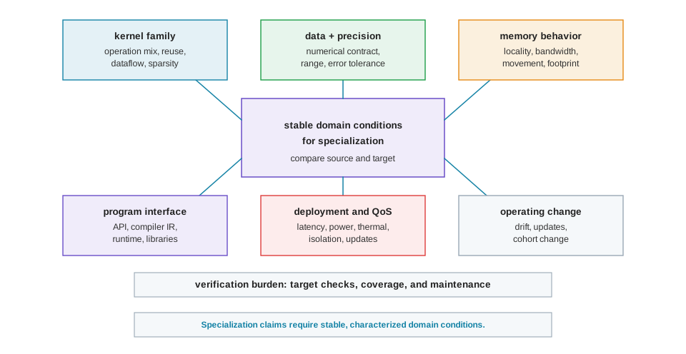
These conditions cleanly separate a stable computation from a usable product path. The kernel family, data precision, and memory behavior dictate whether our computation maintains a stable shape. The program interface, deployment targets, and operating drift dictate whether that shape remains viable beyond an isolated kernel. We treat verification as a distinct endeavor (the work required to prove that these conditions hold true under pressure). For our Lighthouse target, we rely on an executable compiler and interface check to measure offload granularity, latency, memory traffic, and bandwidth against our trace-backed workloads. While a weak condition does not automatically disqualify specialization, we must account for the resulting flexibility, fallback mechanisms, and verification efforts in our final product-path comparison.
9.5.2 Offloading Bounds
Accelerator speedups mean very little if data movement and software invocation overhead consume the savings. We expose that product-path condition with a dimensionally explicit LogCA-style bound. LogCA is a five-parameter model of host-accelerator offloading, covering latency, overhead, granularity, computational index, and acceleration (Altaf and Wood 2017). Our simplified construction uses a payload of \(g\) work units, a host cost of \(C_h\) cycles per work unit, fixed invocation overhead \(o\) in cycles, local compute acceleration \(A\), transferred data \(d\) in bytes per work unit, link bandwidth \(B\) in bytes per cycle, and an overlapped transfer interval \(T_{\mathrm{overlap}}(g)\) in cycles. The host and accelerator times are
\[ T_{\mathrm{host}}(g) = C_h g, \qquad T_{\mathrm{acc}}(g) = o + \frac{C_h g}{A} + \max\left(0,\frac{d g}{B} - T_{\mathrm{overlap}}(g)\right). \]
Our resulting speedup bound is
\[ S(g) = \frac{C_h g}{o + C_h g/A + \max\left(0,\, d g/B - T_{\mathrm{overlap}}(g)\right)}. \tag{9.1}\]
In Equation 9.1, fixed startup cost and data-transfer time share the same unit as host and accelerator compute time. The construction combines the serial-fraction argument of Amdahl (1967) with an explicit communication term. Excessive accelerator invocations (\(N \cdot o\)), driver context switches, or transfer time (\(d g/B\)) can erase a local compute gain. For our Lighthouse target, an implementation-readiness study must measure whether trace-backed spatial-tracking work reaches the array with a granularity and locality compatible with the 3 W power budget.
Figure 9.3 shows how startup and transfer costs shift the offload break-even point. For the illustration, we normalize \(C_h\) to one cycle per work unit, set transfer overlap to zero, hold \(A=100\times\), and sweep pairs of fixed overhead \(o\) and transfer cost \(d/B\). The three pairs are \((2,0)\), \((40,0.005)\), and \((1500,0.05)\), with all time quantities expressed in normalized cycles. Only the break-even structure carries meaning. An offload helps after \(g\) becomes large enough to amortize launch and transfer costs.
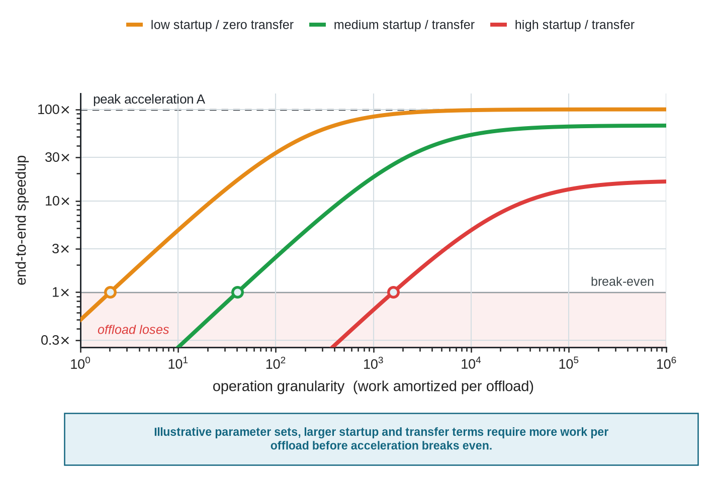
These curves apply progressively larger startup and transfer costs against a fixed 100x local compute acceleration. The low-startup, zero-transfer case breaks even after little work per offload. Medium and high costs require larger payloads before the offload helps, and a nonzero transfer term lowers the asymptotic speedup. Under the illustrative high-cost parameters, the curve approaches about 17x rather than the local 100x ceiling. These are constructed interface costs, not measurements of a named attachment. A strong local result can vanish once the product path charges the actual invocation and data-movement costs.
Offload granularity and operational intensity bound different aspects of performance. Increasing \(g\) amortizes the fixed launch cost \(o\). Roofline defines operational intensity as operations per byte moved; it is a property of the workload and realized data path, not a quantity derived from bandwidth (Williams et al. 2009). If one work unit represents one operation, then \(d=1/\mathrm{OI}\) bytes per work unit and transfer time is \(d g/B\). Changing \(B\) changes that time and the bandwidth roof, while leaving the kernel’s operational intensity unchanged. A kernel whose operational intensity falls below the hardware balance point remains bandwidth-bound even after launch cost is amortized. A target study must therefore measure invocation cost, bytes moved per unit of useful work, available bandwidth, and realizable overlap separately.
9.5.3 Executable Software Path
These architectural bounds only matter if the software stack can realize the offload without mangling its meaning. The lowering path forms a narrow waist (Figure 9.4). High-level domain-specific ASTs (Python or Triton DSLs) descend through mid-level CDFGs (MLIR dialects) and LLVM IR to a point where workload intent meets the selected architectural mechanism, whether a CPU ISA extension or an NPU tensor dataflow engine, and hard silicon constraints. The path then widens into machine-code generation, runtime execution, and verification checks. Lowering is therefore not a passive translation step but the bottleneck where hardware constraints and workload requirements must be jointly qualified for performance, correctness, portability, and maintainability.
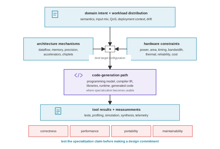
To make this execution path concrete, consider how a high-level Triton JIT block operation lowers into RISC-V Vector (RVV 1.0) primitives. A developer expresses block-parallel elementwise vector operations in Python using Triton’s JIT compiler decorator (Listing 9.1).
import triton
import triton.language as tl

@triton.jit
def add_kernel(x_ptr, y_ptr, z_ptr, N, BLOCK_SIZE: tl.constexpr):
    pid = tl.program_id(axis=0)
    block_start = pid * BLOCK_SIZE
    offsets = block_start + tl.arange(0, BLOCK_SIZE)
    mask = offsets < N
    x = tl.load(x_ptr + offsets, mask=mask)
    y = tl.load(y_ptr + offsets, mask=mask)
    z = x + y
    tl.store(z_ptr + offsets, z, mask=mask)
During compilation, Triton’s MLIR pipeline passes the block representation from high-level ASTs through structured CDFGs down to LLVM IR; a RISC-V backend would then lower the block operations into RVV 1.0 vector primitives, a CPU-targeting path that as of this writing exists only as experimental community work rather than a mainline shipped flow.
Failure mode: The un-amortized offload wall
The mechanism. Because the runtime invokes the NPU through kernel-mode driver calls for each small layer (payload \(g=500\) operations), launch latency (\(o=1500\) cycles) dominates execution before any DMA descriptor setup is even counted. Instead of \(100\times\), the modeled system runs at \(S(g) = 0.33\times\), slower than baseline scalar execution.
The lesson. Local compute acceleration (\(A\)) cannot overcome unamortized startup (\(o\)) and transfer (\(d g/B\)) costs. Offload mechanisms must be co-designed with compiler layer fusion so that payload size \(g\) stays well above the break-even threshold.
Assembly and vector loops provide explicit control over hardware execution, but we must also ensure that higher-level compiler paths generate equivalent code semantics. The kernel below is an author-constructed illustration of the RVV 1.0 stripmining pattern, not captured compiler output.
# RISC-V Vector (RVV 1.0) 32-bit floating-point vector addition kernel
# a0 = x_ptr, a1 = y_ptr, a2 = z_ptr, a3 = element count N
.Lloop:
    vsetvli t0, a3, e32, m8, ta, ma  # Set vector length for 32-bit elements, 8x register grouping
    vle32.v v8, (a0)                  # Load vector x (x_ptr + offset)
    vle32.v v16, (a1)                 # Load vector y (y_ptr + offset)
    vfadd.vv v24, v8, v16             # Vector floating-point addition (z = x + y)
    vse32.v v24, (a2)                 # Store vector z (z_ptr + offset)
    sub     a3, a3, t0                # Decrement remaining element count N
    slli    t1, t0, 2                 # Byte offset = elements processed x 4 (e32)
    add     a0, a0, t1                # Advance x_ptr by processed bytes
    add     a1, a1, t1                # Advance y_ptr by processed bytes
    add     a2, a2, t1                # Advance z_ptr by processed bytes
    bnez    a3, .Lloop                # Loop while N > 0
End-to-end compiler, runtime, interface, and performance claims remain incomplete until workload semantics pass through those transformations and the resulting executable runs on the declared target. Other architecture claims may be supported by different evidence. For the Lighthouse architecture, the target study would add a compiler-generated interface check and an end-to-end execution run that checks correctness while measuring array-cycle ordering, latency, traffic, and bandwidth against a target configuration that still must be pinned. Portability claims would additionally require successful rebuilding and execution across the compiler, runtime, library, interface, and hardware changes named in their scope.
This executable path does not represent an exhaustive system-software inventory. Our target architectures will routinely depend on a complex web of operating-system services, device drivers, firmware, memory management units, synchronization primitives, and deployment configurations. We cannot allow a localized kernel benchmark to conveniently bypass the very infrastructure required to validate its performance claims. Our target studies must retain both the hardware context and the lowering path. We must record the kernel structure, the execution schedule, the compiler (Triton, LLVM) and runtime versions, applicable driver and firmware states, the exact interface, and the specific hardware revision that produced every single result.
We emphasize this hardware-interface boundary because an architectural candidate can look strong in isolation yet collapse once we account for compiler inefficiencies, data movement, and the full end-to-end path. We often see generated blocks that post large isolated kernel speedups, only to discover that our compiler cannot sustain sufficient instruction and data throughput to the execution units, memory traffic dominates the execution time, and only fragile, hand-tuned assembly can ever achieve peak theoretical performance. To protect our designs, our target studies must fully integrate the interface and software paths, mandating a compiler-generated end-to-end measurement before we ever promote a hardware candidate. Our final executable must preserve our intended numerics, memory-ordering semantics, application binary interface (ABI), device-interface contracts, and core workload meaning. If our compiler fast-path subtly mutates the computation just to hit a performance target, we have not achieved a transferred speedup. We have simply broken the application.
Once we make this end-to-end product path explicitly defined, we can finally ask whether a lightweight source screening check can cull our worst ideas early, reducing our reliance on expensive full-system evaluations without altering our ultimate architectural decisions.
9.6 Cheap Screening Proxies and Pre-Filters
Inexpensive proxy checks can significantly accelerate design space exploration, but only within the exact coverage regions where their ordering predictions remain validated. We must explicitly define the check invariant, its valid support region, and the separate high-fidelity target reference we evaluate against. Modeling the relationship between validated coverage and overhead establishes the efficiency bounds for deploying cheap screening tools across our target stream.
9.6.1 Coverage vs. Overhead
Screening proxies reduce evaluation latency by filtering out unpromising candidates early, balancing cheap pre-filter accuracy against the heavy cost of high-fidelity signoff tools. In our methodology, service work means the expected evaluation effort required per target comparison, explicitly excluding queueing delay. We model this workflow using an Amdahl-like service-work formulation (Amdahl 1967). Let \(c_{\mathrm{hi}}\) represent our mean service cost for extracting array-cycle ordering from compiler-connected RTL simulation or gem5 full-system runs, and let \(c_{\mathrm{cheap}} < c_{\mathrm{hi}}\) be the mean cost for our SCALE-Sim screen. We define \(f\) as the validated coverage, representing the fraction of target comparison mass where the screen’s ordering successfully settles the advance decision within declared error limits without requiring escalation.
Let \(a\) be the fraction of target comparison mass submitted to the cheap check (\(f \le a\)). We model our multi-tier evaluation pipeline using selective classification screening math, expressing our overall screen service-work speedup \(S_{\mathrm{screen}}\) as follows.
\[ S_{\mathrm{screen}} = \frac{1}{(1-f) + a \cdot (c_{\mathrm{cheap}}/c_{\mathrm{hi}}) + \epsilon} \le \frac{1}{(1-f) + f \cdot (c_{\mathrm{cheap}}/c_{\mathrm{hi}}) + \epsilon}. \tag{9.2}\]
In Equation 9.2, \(\epsilon \ge 0\) captures normalized per-item routing, auditing, and rework overhead. This inequality holds because \(f \le a\); we cannot settle a case without executing the check. We achieve maximum speedup when every cheap check executed settles the case (\(a = f\)).
As \(c_{\mathrm{cheap}}/c_{\mathrm{hi}} \to 0\) and \(\epsilon \to 0\), the theoretical free-check ceiling approaches \(1/(1-f)\). This bound demonstrates that validated coverage \(f\), rather than screening speed alone, sets the maximum obtainable speedup. Borrowing from selective classification theory (El-Yaniv and Wiener 2010), abstaining from uncertain or out-of-support predictions avoids false acceptance but forces un-settled candidates to incur full \(c_{\mathrm{hi}}\) reference evaluation costs. If we estimate coverage solely on accepted cases, we introduce sample-selection bias (Heckman 1979); thus, \(f\) must be evaluated across representative samples of the entire target stream.
9.6.2 Efficiency Bounds
Figure 9.5 maps validated coverage against review speedup for three cost ratios (\(c_{\mathrm{cheap}}/c_{\mathrm{hi}}\) of 0.01, 0.1, and 0.3), each shown for an ideal router that pays for the cheap check only where it settles a case (\(a=f\)) and for full screening (\(a=1\)), against the free-check ceiling \(1/(1-f)\). The lesson sits at the annotated point: at \(f=0.6\), coverage caps the speedup at \(2.5\times\). Lowering the cheap-check cost only pushes performance toward that ceiling; expanding validated coverage \(f\) is the only way to raise it.
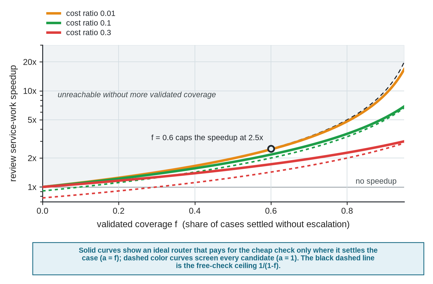
When we isolate our validated coverage from routing, auditing, and rework overheads (\(\epsilon = 0\)), the curves in Figure 9.5 reveal the fundamental bottleneck of surrogate screening. Our solid curves represent an ideal scenario where we pay for the cheap check only when it successfully settles the comparison, while the corresponding dashed curves assume we pay to screen cases that subsequently escalate. Every comparison falling outside our validated coverage still incurs the full compiler-connected RTL reference cost. At \(f = 0.6\), even a hypothetical free check cannot push our speedup past \(2.5\times\) in this model. Consequently, when we claim a screening-work speedup, we must explicitly provide the cost ratio, the class-specific error bounds, and the sampling and confidence calculations backing our coverage estimate. For any consequential architectural decision, we should always report a conservative lower confidence bound on our supported coverage (derived under a predeclared target sampling procedure) rather than relying solely on a fragile point estimate of \(f\).
We must also recognize that this component-level bound does not predict our iteration time or our complete-workflow productivity. Queueing delays, parallel simulation capacity, raw model and tool licensing costs, failed run overheads, and human review cycles all sit squarely outside this specific service-work model. Finally, we must ensure that each transferred result remains attached to the exact hardware and software versions it observed during evaluation.
9.7 Managing Version Dependencies and Interface Contracts
Any transferred hardware-software result remains valid only for the exact version pair that produced it. If we change either the hardware snapshot (such as NPU tensor array dimensions or CPU ISA extension configs) or the software stack (such as Triton 3.0 compiler passes or LLVM 19 lowering targets), that invariant may immediately fail. We cannot requalify one side of the system without recording the other, as doing so destroys the foundation needed to support our target claims.
Any target we evaluate widens our causal chain from a single array parameter out to the compiler, runtime environment, memory hierarchy, and host system. Because of this widened dependency, we must version our hardware and software snapshots together. We also need to continuously check our local, subsystem-level objectives against our overarching Lighthouse system goals to ensure they remain aligned.
We often find that a single-layer optimization can be locally correct while degrading the complete system. In modern cross-layer architecture, our work routinely involves techniques like algorithmic tiling optimized for the memory hierarchy (such as FlashAttention, an IO-aware exact attention algorithm for transformer model speedup (Dao et al. 2022)) and pairing narrow numerical formats with both hardware efficiency and accuracy objectives (such as Microscaling / MX formats, a narrow-precision floating-point block scaling standard for machine learning workloads (Rouhani et al. 2023)). Take our Lighthouse system as an example. Both the compute capability (RVV vector units or NPU tensor array) and the camera-interface bandwidth must work together to support the target frame rate. If we hold either the hardware or software fixed, we artificially restrict our design space and mask critical tradeoffs that a joint design approach would expose. A localized throughput improvement that violates our latency or bandwidth constraints remains unacceptable.
The performance benefits we extract from these cross-layer techniques remain tightly bound to the paired algorithm, chosen numerical format, spatial mapping, software stack (Triton, LLVM), and underlying hardware conditions. The moment we change any single member of this stack, we must reopen and re-verify all of our dependent latency, bandwidth, accuracy, and efficiency claims.
When our software tools return performance signals, those results support a target claim only after we qualify the tests, profiles, and failure data against the precise hardware snapshot and study scope. Because software tuning converges much faster than hardware implementation checks, the two must co-evolve without letting the fast lane overwrite the slow one (Figure 9.6). A fast software result may propose a hardware revision, but that revision reaches the versioned target state only through a shared study record and an explicit decision by its owner. A rapid software speedup can reopen a hardware question without silently bypassing an established validation baseline.
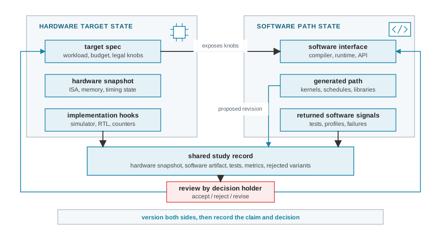
Our hardware target deliberately exposes legal architectural knobs to the software interface, just as our generated kernels and compiler schedules often reveal intense pressure to revise the hardware snapshot itself. The arrow labeled “proposed revision” in our diagram does not change the target state directly. Instead, our shared study record and decision-holder review determine whether that proposed revision actually becomes the new target state. The two outer return paths carry only those accepted, reviewed revisions back to our versioned hardware target and software interface. Consequently, an unexpected fast software result can reopen a hardware design question without silently overwriting our established baseline.
Our figure does not mandate a synchronized, lock-step universal loop. We understand that our hardware and software teams will advance at different rates. Instead, we enforce that each evaluation result remains bound to an immutable hardware-software version pair. Our review process then joins only those claims whose architectural dependencies intersect, rather than forcing us to serialize every minor change through a single fixed development cycle.
In this methodology, we define the software state comprehensively to include the compiler (Triton, LLVM), runtime environment, programming interface, and all generated machine artifacts. If our execution target relies on drivers, embedded firmware, operating-system services, or device control logic, we must version those elements within the same lane.
Our design-time results, production telemetry, and subsequent software enablement phases are scoped to the artifact versions and operating conditions they actually observe; therefore, they support distinct architectural claims. A simulator result explicitly belongs to the candidate design and conditions we evaluated at that moment. Production telemetry belongs exclusively to the shipped hardware-software version and the live deployed workload. Any later compiler or firmware result belongs to its revised software path and the specific hardware version it targets. Our study record binds these returns together while keeping them separately scoped, guaranteeing that a newer optimization signal never silently overwrites an older, foundational result.
When we execute a rollback, we must restore the entire configured dependency set (not just our isolated model weights or software binaries). If a memory schema, numerical representation, compiler, runtime, interface, tool, library, or hardware target has changed, simply returning to an earlier learned component without its exact compatible configuration fails to restore our earlier system state.
Attributed observations from deployment can strongly motivate a new calibration study for our next hardware generation, but they must never automatically update a surrogate model or an architectural design rule. As predictive-uncertainty evaluations demonstrate, accuracy and calibration easily degrade under dataset shift (Ovadia et al. 2019). While this degradation motivates us to implement new target checks, it does not automatically establish architecture correctness, nor does it transfer a complete architecture conclusion. Our calibration study must explicitly bind each observation to the shipped hardware, the exact software stack, the workload cohort, and our measurement conditions. We must keep our calibration cases separate from our held-out checks, and test whether the deployed cohort actually covers our next architectural target. The deployed workload is merely a selected sample of what the earlier system happened to serve. When we reuse a learned predictor, any changed workload or operating-condition distribution becomes a textbook architecture instance of distribution shift. If we fit a model to that shift without fresh target checks, we risk prematurely narrowing our next processor design around yesterday’s traffic.
For instance, NVIDIA reported workload-specific single-node training improvements on the exact same H100 hardware between the MLPerf Training v2.1 preview and v3.0 simply by applying software optimizations, which yielded a 17 percent BERT improvement (Eassa and Eryilmaz 2023). We must view this vendor-reported comparison strictly as an example of continuing software enablement; it does not represent a dependable, compounding improvement rate, nor does it revise our hardware’s fundamental design-time result.
Our five-stage transfer test is what transforms these complex source-to-target differences into a new architectural target study.
9.8 Framing Architectural Pattern Transfer Studies
Applying our five-stage transfer test to our Lighthouse spatial-tracking target exposes how a new design problem reshapes our unit actions and verification demands.
- Compare source and target decisions. Our source study compared five simulated array shapes against a local score ratio of cycles to utilization. The 32 by 32 shape emerged as our local reference. However, our target environment asks a fundamentally different question regarding whether we should freeze an RTL-facing array alongside its compiler-visible tiling and memory interfaces. The workload shift is distributional, while introducing Triton/LLVM compilation, RTL synthesis, memory hierarchies, and physical paths creates sweeping component changes. Because these shifts alter our artifact boundaries and acceptance criteria, the target carries new decision semantics, instantiating a new architectural design problem.
- Separate the source into transfer units. We break down the source architecture into modular transfer units. Historical records, workload definitions, project state representations, proposing methods, our SCALE-Sim screen, tool interfaces, candidate artifacts, and final conclusions each carry distinct invariants and dependencies.
- Identify the affected slice. We trace immediate divergence in the trace-backed workload distribution, compiler mapping strategies, executable paths, process libraries, physical validation checks, and subsystem power targets. While source simulator outputs remain valid as historical data, they miss the implementation properties demanded by our target architecture.
- Assign a target action. We route each unit by reusing historical artifacts, refreshing workload and live project state, re-evaluating target alternatives, and requalifying screening tools. We adapt interfaces and architectural checks, retrain learned components only where target support degrades, and recompose system configurations around new integrations. We replace or retire incompatible components and reject any direct transfer of the source recommendation.
- Require target evidence and test claims of transfer benefit. We pair every changed dependency with a target check capable of observing its specific architectural risk, while enforcing integration checks wherever unchanged components meet modified neighbors. If our study claims a transfer benefit for an adapted unit, we must validate it against a matched target-only baseline, retiring any harmful prior and retaining cost-neutral units only when they improve another declared target criterion.
While these five steps structure our target study, they do not give us the authority to freeze an array or an interface. Until we explicitly declare our legal target candidate set and establish a credible architectural comparator, we cannot run our target comparison. As a result, our target decision remains wide open.
We cannot inherit claims of representativeness, implementation readiness, physical viability, or operational success from the source array’s results. Each target obligation pairs a minimum test with the claim boundary we must accept if that test is absent (Table 9.3), across ten domains from workload coverage and candidate comparison through RTL, physical, containment, and operational-readiness checks. The through-line: every omitted test narrows what we can claim, keeping unverified assumptions out of a generalized system claim.
| Target obligation | Minimum test | Boundary if absent |
|---|---|---|
| Workload coverage | We require trace-backed common and tail cases, strictly versioned and with all exclusions clearly stated. | We can make no representativeness claim. |
| Candidate comparison | We must predeclare the legal target space, search and evaluation budgets, a credible architecture comparator, our decision rule, and a robust sensitivity or resolving-power check. | We can make no claims outside our evaluated candidates, nor any comparative AI-contribution claim if our study cannot distinguish its arms. |
| Transfer benefit | When we claim that transfer helps, we must compare the adapted component against a target-only arm sharing the same tasks, data, tool access, budgets, and stopping rules (without the source unit). We must explicitly count adaptation, requalification, integration, use, checking, and retirement costs. | We forfeit any transfer-benefit claim. We must retire a harmful source prior, retaining a cost-neutral one only if it improves another declared target criterion. |
| Mapping and software path | We demand compiler-generated (Triton, LLVM), end-to-end execution using pinned mappings, compilers, runtimes, CPU ISA extension configs (RVV), driver and firmware versions (where applicable), and strictly defined interface versions. | We cannot claim our array is usable by the target software stack. |
| Interface and memory cost | We must measure offload granularity, bandwidth, traffic, and latency using LogCA and Roofline models, alongside a calibrated energy-and-power model that captures execution rates, duty cycles, leakage, idle power, and the complete subsystem boundary. | We forfeit any 3 W power or system-speedup claims. |
| Cheap-screen validity | We must check representative target samples against a separate property-specific reference path (gem5, Verilator), enforcing class-specific error limits, uncertainty measures, the ability to decline unsupported predictions, and a subsequent drift audit. | We relegate SCALE-Sim to a source-study tool rather than a valid target decision filter. |
| RTL behavior | We need independently derived reference tests where practical, alongside lint, functional simulation using Verilator, synthesis via Yosys, and formal property verification using Cadence Jasper and SystemVerilog Assertions (SVA). We must also add fault and threat models specifically required by our target architecture. | We can make no implementation-readiness, reliability, or security claims beyond the specific properties we checked. |
| Physical behavior | We must pin our 3 nm-class low-power process design kit, libraries, and PVT conditions; then we test area and floorplan feasibility using OpenROAD, static timing closure using OpenSTA, setup and hold corners, congestion, routed dynamic and leakage power, power delivery, and electrothermal behavior using Ansys RedHawk-SC. | We surrender any signoff, tapeout, or physical-feasibility claims. |
| Containment | We must exercise every proposed bypass, disable function, guardband, isolation mechanism, or fallback against the specific fault or attack it is designed to contain. | We cannot claim that our implementation will contain or recover from that failure. |
| Operational readiness | We must confirm required tool access, have our qualified operators challenge representative target cases within our allocated review capacity, and permanently record our named decision authority. | We cannot claim that our transferred workflow is operable, challengeable, or capable of supporting a target commitment. |
Our workload coverage and candidate comparisons ultimately frame the target architecture question. The concept of transfer benefit stands separate; we apply it only when our study argues that transferring a source structure provides a tangible advantage over building a target-only version. If we claim that an AI-native workflow, rather than point AI assistance, gives us an edge, we must back it up with the matched, complete-workflow comparison detailed in Chapter 10. From there, our executable paths and interface costs prove whether our candidate architecture can actually run. Finally, our cheap-screen, RTL, physical, containment, and operational-readiness checks draw strict boundaries around what our target results can legitimately support.
Three representative scenarios show the five-stage test scaling across domains (Table 9.4): a constructed physical-design case (a learned congestion predictor evaluated across shifting process design kits), a vendor-reported software case (NVIDIA H100 optimization gains across MLPerf releases), and a physical silicon-defect case (Intel Cougar Point SATA degradation). Across all three, the valid action follows the nature of the broken dependency, and every transferred component still demands a target check matched to its own failure mode. The first case is one we constructed ourselves. While CircuitNet (an open-source dataset and benchmark for IC physical design) supplies congestion-prediction data and tasks (Chai et al. 2022), and ChiPBench (an end-to-end physical placement benchmark suite) offers physical placement and PPA evaluations (Zhihai Wang et al. 2025), neither source natively reports the combined transfer procedure we outline here. Our other two cases tackle the realities of continuing software optimization on fixed hardware, and a severe physical silicon defect that no software patch could ever resolve.
| Transfer unit | Changed dependency | Valid action | Required target check |
|---|---|---|---|
| Our constructed transfer case for a learned congestion predictor trained on one specific process, library, and design family | Our target process, standard cell library, netlist family, placement flow, or routed-result definition shifts. | We must first requalify the unchanged predictor; we only recalibrate, adapt, retrain, or retire it after isolating exactly what no longer holds. | We must measure class-specific target errors and decision quality against routed target results that we keep strictly isolated from our calibration or training data. |
| H100 software-optimization results reported between MLPerf Training v2.1 preview and v3.0 (Eassa and Eryilmaz 2023) | A subsequent compiler (Triton, LLVM), library, workload, or hardware generation alters our paired configuration. | We must constrain the published improvement to its explicitly reported versions and workloads; we then rerun the comparison for our new architectural pair. | We must repeat the end-to-end workload measurement, explicitly pinning both hardware and software versions while maintaining the exact same result definition. |
| Cougar Point containment and correction results (Intel Corporation 2011) | Our target defect and the specific mechanisms capable of reaching it differ. Intel’s permanent correction required revised silicon alongside repair or replacement; they did not present a firmware-only fix. | We cannot assume a firmware-only remedy will resolve a deep silicon defect; we must deploy a correction or containment mechanism structurally matched to the failure. | We must exercise the corrected silicon and any proposed containment strategies against our target failure class before we ever claim a correction. |
When examining the learned-predictor case, we ensure that a familiar model name never blindly substitutes for target support. Our H100 case preserves the integrity of the reported result, stopping us from improperly extrapolating a specific 17 percent gain into a generalized software-improvement rate. The Cougar Point case underscores lessons about failure reach, reminding us that we cannot assume every silicon defect will succumb to the same architectural remedy. Across all three examples, we retain valuable source knowledge while refusing to stretch our conclusions beyond the specific configurations that produced them.
Transferring these components does not alter our core decision rights. While we allow automated components to propose or screen candidates within the boundaries of our declared study, the primary responsibilities (rejections, waivers, the final architecture freeze, physical signoff, and tapeout) remain firmly in the hands of the named architectural roles we defined in Chapter 11.
At this stage, our adaptation decision is complete, even though our ultimate target architecture decision remains unresolved. We have effectively paved the way for our study structure and reference candidate to move forward. However, the original source conclusion simply cannot transfer to the target context.
9.9 Common Pitfalls
Adapting legacy microarchitectures, surrogate models, or offload patterns into new systems without explicit transfer contracts introduces severe architectural risks. As we execute design transfers, we frequently fall into critical traps regarding conclusion transferability, LogCA offload bounds, selective requalification scopes, and transfer map construction.
Transferring source conclusions without requalifying target artifacts. Assuming that a performance win, optimization ratio, or trade-off conclusion validated on a source process node or workload automatically holds in a new target context. While source candidate identities and execution scripts can be transferred, microarchitectural conclusions do not transfer across boundary shifts in standard cell libraries, ISA lowerings such as Triton to RVV 1.0, or memory controllers.
Violating LogCA offload bounds in accelerator design. Evaluating host-to-accelerator offload patterns using simplified execution speedup estimates while ignoring the communication terms that LogCA-style models make explicit (Altaf and Wood 2017). Architectural models that omit latency, overhead, and transfer granularity across PCIe or CXL interconnects yield unrealistic offload efficiency metrics, concealing DMA setup costs and host-side synchronization stalls.
Conflating limited requalification with decision reformulation. Failing to distinguish between updating dependent checks under localized drift versus reformulating a fundamentally altered design decision. Treating shifted objective semantics or new packaging constraints as minor parameter drift leads to improper model recalibration, while treating minor workload adjustments as ground-up redesigns wastes compute on redundant verification.
Misapplying selective classification math to cheap-screen surrogates. Utilizing fast learned surrogates for candidate screening without establishing selective classification coverage and error bounds (El-Yaniv and Wiener 2010). Evaluating cheap proxy models without defining explicit abstain thresholds or computing coverage-dependent error rates causes surrogates to issue high-confidence predictions in out-of-distribution design regions, steering candidate selection toward flawed microarchitectures.
Evaluating transfer benefit against unmatched baselines. Claiming architectural improvement from an AI-native or transferred workflow by comparing it against an unoptimized or mismatched target baseline. An authentic transfer evaluation requires comparing the ported design against an equally tuned target-only baseline while fully accounting for adaptation overhead, verification contracts, and physical signoff costs.
9.10 Open Questions
The true frontier of architecture reuse lies not in the mechanics of packaging components, but in bounding their expiration. As we have established throughout our discussions, physical implementations, software stacks (Triton, LLVM), and integration constraints shift between design problems. When left unchecked, this architectural drift turns reuse into a source of silent system failure rather than an efficiency gain. Until we can resolve when a prior architectural conclusion has expired and safely transfer verified state, we expect manual requalification to remain the bottleneck.
Dependency maps and minimal requalification sets. Isolating affected design slices requires dynamic dependency mapping to prevent indiscriminate re-testing or silent failures.
How can we identify the minimal safe set of components to requalify after a hardware or software change? Hidden dependencies can easily make a partial re-test look sufficient while leaving an invalid architectural claim untouched. An AI-native design system must be capable of mapping complex system-wide dependencies to pinpoint the exact subset of claims affected by a given change, achieving the safety of full cross-layer requalification while requiring only a fraction of target checking.
At what point does a system change create a new design problem rather than limited requalification? A shifted objective or a new set of design constraints can invalidate our original design question, even if many of the underlying artifacts still match. We need reliable methodologies to determine exactly which prior claims remain relevant, and when a change is so fundamental that it demands a newly formulated design study from the ground up.
Transfer invariants and offload generalization. Predicting design transferability relies on robust invariants that bound host-accelerator offload efficiency under shifting interconnect topographies.
Which invariants predict whether a learned architecture component is worth transferring? Simply looking at a model’s accuracy on the source task is rarely enough, because preserved behavior can still silently fail under changed target conditions. As architects, we need robust invariants that can reliably predict target decision quality and estimate requalification costs far better than naive metrics like source accuracy or basic source-target similarity.
How do we bound host-accelerator offload efficiency under shifting interconnect topographies and compiler tile schedules? We must establish analytical LogCA bounds that automatically update offload thresholds across transferring hardware topologies, preventing inefficient host-to-accelerator offload dispatches.
9.11 Summary
Our five-stage transfer test converts source-to-target differences into a new architectural study: we assign a target action to each unit (whether carrying forward unchanged components, updating representations, or retiring stale priors) and pair every changed dependency with a target check capable of observing the resulting risk. When we apply this framework to our Lighthouse study across all eight prompt stack layers, we treat retained simulator telemetry and candidate identities strictly as historical baselines. We systematically refresh our workload, ISA contracts, compiler toolchains, timing models, process parameters, power envelopes, and formal verification checks, refusing to let local source recommendations substitute for physical implementation evidence.
When we evaluate pattern transferability across Architecture 2.0, four core takeaways govern our work.
Key Takeaways: What Transfers and What Must Be Requalified
- Invariant preservation. Data sources, models, tool paths, or verification checks remain reusable strictly while core invariants and underlying dependencies hold for the target context.
- Selective requalification via transfer maps. Structured transfer maps partition system dependencies, forcing fresh target checks and LogCA offload bound verifications whenever workload, compiler, process library, or constraint boundaries shift.
- Integration check enforcement. Dedicated integration checks are required whenever an unchanged component interfaces with a changed neighboring block, preventing correlated system failures across decoupled boundaries.
- Conclusion isolation. Historical source records carry forward as valuable provenance, while prior architectural conclusions remain isolated and withheld until newly established target evidence confirms them in the new design context.
As we transition into the next chapter (Chapter 10), we hand off this source-to-target map and our versioned hardware-software state to address a broader question. Across repeated and varied architectural studies, does our configured AI-native system actually improve the final hardware result, reduce the total engineering cost of achieving it, or deliver on both fronts?