
5 Prediction, Generation, and Optimization
“Data can tell you that the people who took a medicine recovered faster than those who did not take it, but they can’t tell you why.”
— Judea Pearl and Dana Mackenzie, The Book of Why (2018) (Pearl and Mackenzie 2018)
Pearl, Judea, and Dana Mackenzie. 2018. The Book of Why: The New Science of Cause and Effect. Basic Books.
Author’s Note. Judea Pearl’s insight highlights the central challenge in choosing AI architecture methods. Statistical surrogate models and generative search loops can rapidly surface high-scoring candidates, but raw correlation cannot explain the underlying physical hardware mechanism. As architects, we must pair predictive search with an understanding of the underlying physical mechanism, not just correlation with it.
North-Star question
Which engineering job requires assistance, is AI assistance truly warranted, and what is the smallest sufficient approach that still retains a named check and a reliable fallback?
When we choose an approach, we must start with the architecture problem itself, not the model. If our cache study has three legal capacities and we can evaluate each affordably, we run our direct tools to settle the comparison. Conversely, if thousands of existing configurations compete for a few expensive simulations, we might use a predictor to screen them or an optimizer to select which ones to run. And if our required RTL, test, kernel, or compiler schedule does not yet exist, we can rely on generation to construct a candidate. These are different jobs, and we must treat them accordingly.
We see this same distinction inside larger systems. We might use a foundation model to supply reusable prior knowledge, lean on retrieval for our current project context, and let an agent request tools and react to their returns. Yet, those components do not form new peer method families, and none of them makes generation the automatic default. As architects, we still have to decide which operation our job actually requires. We must determine whether a conventional, learned, or hybrid technique should perform it, whether we need to compose several components, or whether direct tool use is already enough.
Finding the right fit depends on much more than our desired output. Our available data, legal search space, evaluator limits, feedback cost, and runtime latency can all change the answer, along with confidentiality constraints, required reliability, reversibility, and the consequence of failure. For instance, a method that saves simulator calls might still lose out once we account for model setup, licensed tools, validation checking, and expert review. Likewise, a capable generator can be the wrong choice if a compiler pass or parameterized template already constructs our artifact safely.
Our most durable rule is to always choose the smallest sufficient approach. We should name the engineering role first, choose a method family and concrete technique only when they fit, and always keep a real evaluator or check ready to reject the output. If we force a poor fit, we risk flooding a saturated evaluator with generated artifacts, pushing a predictor outside its support, or blowing our evaluation budget optimizing a proxy. Therefore, our choice must explicitly define the allowed work, tool roles, cost envelope, checks, fallbacks, and stopping conditions.
As the second technical building block of Architecture 2.0, prediction, generation, and optimization methods define our search strategy, required tools, budget, and checks. However, methods alone do not supply the runtime environment, nor do they determine what a returned measurement can establish. To execute our selected methods reliably within an automated workflow, we must connect them to tool-connected execution environments in Chapter 6.
Learning objectives
This chapter establishes the following learning objectives:
- Distinguish between architecture engineering roles, method families, and concrete techniques.
- Select the minimal, most sufficient approach constrained by available budget and checking capacity.
- Appropriately match prediction, generation, and optimization to the required limiting work.
- Compose discrete components while maintaining explicit tool checks and viable fallbacks.
5.1 Optimization Roles and Method Families
When we attempt to accelerate hardware design with algorithmic search or learned models, we risk confusing the engineering job we need done with the tool we use to perform it. In architecture studies, our primary goal is rarely to deploy sophisticated algorithms for their own sake; it is to construct missing artifacts, estimate expensive physical consequences, search large decision spaces, or check claimed properties. Decoupling these functional engineering roles from their underlying method families forms our first line of defense against unnecessary complexity. If we already know our candidate configurations and can evaluate them affordably, adding a predictor, generator, or optimizer creates setup overhead and verification backlog without removing our actual bottleneck.
We prefer the smallest sufficient approach, defined as the least elaborate method that performs the required engineering job while preserving our evaluator and later checks. This strategy minimizes our total effort rather than just shortening the code or reducing inference cost. We consider choosing “no added method” a positive engineering decision whenever direct evaluation costs less and maintains our required checks.
Consider the three cache capacities we specified for our prospective Lighthouse cache study. Because we simply need to compare known candidates, direct evaluation fits our declared budget perfectly. If our study instead contained thousands of microarchitectural configurations (such as sizing CPU instruction windows or NPU tile factors), evaluating each candidate directly in simulators like gem5 (a cycle-accurate microarchitectural simulator), Sniper (a parallel multi-core simulator), SCALE-Sim (a systolic-array accelerator simulator), or Ramulator (an open-source cycle-accurate DRAM simulator) would quickly exhaust our computing budget. We might then choose to screen candidates with a regression model or surrogate. We would first need to qualify that model against stronger reference results from our same workload and design region before passing its ranked finalists to our simulator and physical checks. Expanding our choice space shifts the limiting work, which may in turn change our approach.
If we jumped straight from our cache comparison to a favored mechanism, we would hide the actual work required. Making our design decisions explicit means separating the engineering role, method family, technique, and system composition, then evaluating them in sequence so that our engineering goal dictates the operational method family. That family in turn selects a concrete conventional, learned, or hybrid technique before we compose multicomponent pipelines (Table 5.1).
| Decision layer | Question | Choices | Required discipline |
|---|---|---|---|
| Engineering role | What work must we do? | Propose, screen, search, critique, repair, check, explain, or coordinate. | We must name the input, expected output, limits, and next check for each role. |
| Method family | What broad operation performs the role? | Prediction, generation, optimization, or another operation our problem requires. We treat these families as useful but not exhaustive, and we may combine them. | We select the operation from our required output and feedback rather than forcing a fixed sequence. |
| Technique | What concrete mechanism fits our artifact and feedback? | A conventional, learned, or hybrid technique, such as an analytical model, regression, Gaussian process, graph neural network, large language model, Bayesian optimizer, solver, compiler pass, or heuristic. | We state the assumptions, applicable conditions, cost, and failure conditions of the actual technique. |
| System composition | Which components must work together? | One technique and a tool, or several generators, predictors, optimizers, conventional and learned techniques, retrieval components, and tools. | We give every component a distinct input, output, cost, and check. |
When we use prediction, we estimate a property or later state; with generation, we construct an artifact or candidate; and through optimization, we select among actions or candidates. We use the terms “conventional,” “learned,” and “hybrid” to describe how a concrete technique performs one of these operations. Hybrid techniques often take a neurosymbolic form by pairing probabilistic neural models with symbolic logical systems, Abstract Syntax Tree (AST) type checkers, Control-Data Flow Graphs (CDFGs), compiler Intermediate Representations (IRs), or analytical models. In this formulation, probabilistic generators or surrogates propose candidate structures while symbolic logic engines enforce hard invariants. While foundation models, retrieval components, and agents might support or coordinate our work, we view them as components inside a composition rather than peer method families.
This separation also preserves our direct-tool path. When we decide on no added method, it means our declared tools already perform the needed work economically and reliably, even if a tool’s internals happen to include learning. A strict no-AI path relies entirely on conventional methods and tools. We recognize that either choice can serve as the smallest sufficient approach. Our functional engineering roles connect to verified execution paths across the pipeline stages (Figure 5.1).
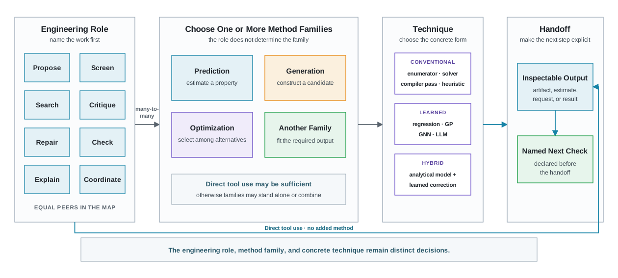
An engineering role cannot select a method family by itself (Figure 5.1). Each of the eight roles (propose, screen, search, critique, repair, check, explain, and coordinate) can reach either an unaugmented tool path or any of prediction, generation, and optimization through a many-to-many mapping. Each family in turn admits concrete conventional, learned, or hybrid techniques such as regression models, language models, or Bayesian optimizers. Our proposals do not necessarily need generation, our screening processes do not always demand prediction, and our searches do not require a learned optimizer. What matters is whether the output remains inspectable and whether our named check can reliably reject or redirect it, since every path ends in exactly that pairing.
We find that our costs always follow the missing work. When a generator proposes missing RTL or a testbench, it adds checking work. When a predictor screens existing candidates, it introduces new qualification and confirmation tasks. If an optimizer selects among too many legal configurations, we must give it a declared objective and spend part of our evaluation budget on the search itself. While these conditions might suggest a particular family, they do not automatically select a concrete technique for us. Our limiting work and its specific conditions determine the best fit; once we make that work visible, we can choose our approach without letting an arbitrary component name drive our decision.
5.2 Anchoring Optimization Method Selection
Every algorithmic enhancement in computer architecture comes with an invisible invoice covering the data collection, surrogate qualification, hyperparameter tuning, and verification checking required to keep it trustworthy. Before committing scarce computing cycles and engineering effort to an advanced prediction, generation, or optimization method, we must verify that the added machinery relieves a genuine bottleneck rather than shifting our workload into a saturated verification pipeline. Grounding our method selection in physical constraints prevents us from adopting elaborate frameworks that offer nominal speedups while inflating total study cost.
To keep our selection process transparent, we establish a pre-flight evaluation protocol. This protocol evaluates our architectural goals alongside conventional baselines, forcing us to identify the precise limiting work before authorizing an advanced technique.
5.2.1 Pre-Flight Evaluation Criteria
Before authorizing any algorithmic optimizer or learned surrogate, we pass the prospective study through six pre-flight criteria. These criteria test whether direct tool execution or a conventional heuristic can resolve our architectural question before we introduce added methodology.
State our architecture decision, comparator, objectives, constraints, and the concrete output our work must produce.
Ask whether direct evaluation, a conventional algorithm, solver, compiler analysis, heuristic, or parameterized generator can settle the question within our available budget.
Identify the limiting work. Candidate construction points us toward generation; expensive outcome measurement points toward prediction; selecting among too many legal alternatives points toward optimization.
If actions change later state, we must decide whether we need a transition-aware predictor or sequential optimizer. We should not introduce either when we can evaluate candidates independently.
If measurement, checking, or review is already our bottleneck, we need to improve that path or reduce the work arriving at it. Producing more candidates cannot repair a saturated evaluator.
Reject the proposed method when its data, representation, legal actions, evaluator, support, total cost, fallback, or stopping condition is inadequate.
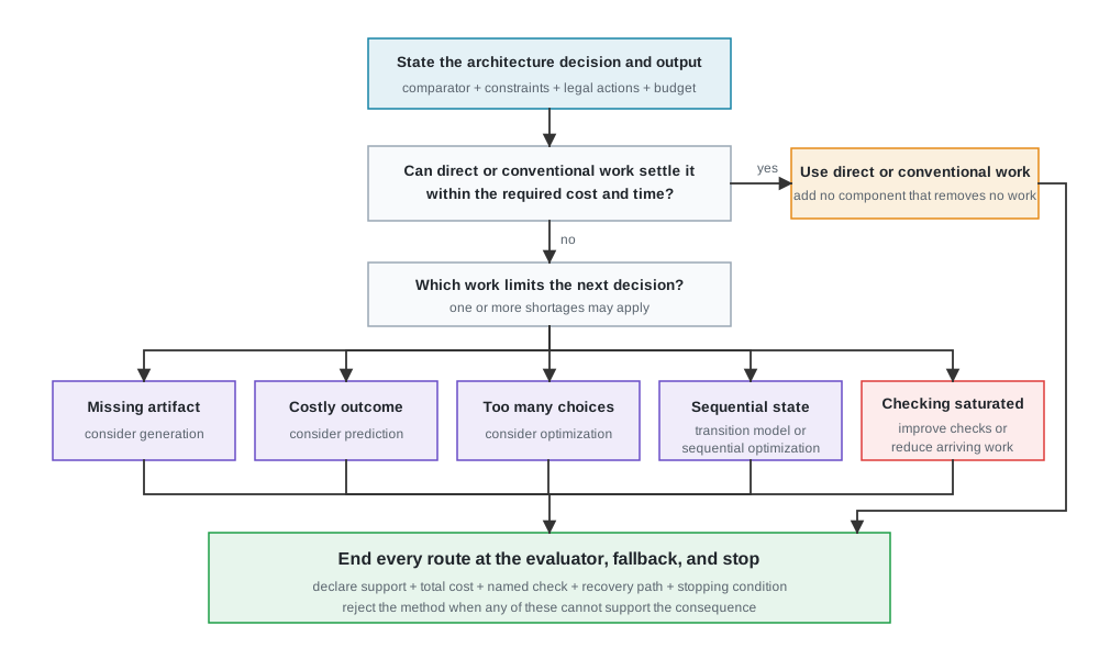
Our pre-flight tests compose into a decision tree for approach selection (Figure 5.2). We start from the architecture decision and required output and first test whether direct evaluation or a conventional method settles the question within budget; only when direct tools prove insufficient does the specific bottleneck point elsewhere. Candidate shortages point to generation, expensive outcome measurements to prediction, and expansive decision spaces to optimization, while actions that alter subsequent system states call for transition-aware predictors or sequential optimizers. A saturated checking path calls for throttling candidate arrivals or upgrading evaluator efficiency rather than generating more candidates. Every route ends at declared support, total-cost justification, a named check matched to physical consequences, a fallback, and a stopping rule, and we justify a composition only when each component removes distinct limiting work while preserving those safeguards.
Fit alone does not make an approach usable. Before we commit engineering resources, we need an explicit checklist that compares direct tool paths against added method compositions on equal footing (Table 5.2). Each of its nine attributes, including job definition, inputs, output, search space, evaluator rigor, total cost, confidentiality, reliability, and stopping rules, pairs with a concrete preselection question. Requiring every proposed method to answer those questions up front prevents comparisons among vague algorithm names and grounds every technical path in physical feasibility and cost.
| Attribute | Question to answer before selecting the approach |
|---|---|
| Job and question | Which limiting work will this approach remove, and must we construct, estimate, select, or establish a property? |
| Inputs and support | Which represented state, artifacts, observations, workloads, design regions, and process assumptions may we use? |
| Output | What concrete result will our method return? |
| Search and allowed actions | What structure does our legal space have, and which elements or artifacts may the method change or request? |
| Evaluator and later checks | Which evaluator can reject a bad output, what does it observe, and which stronger checks remain? |
| Cost and latency | What setup, predictor qualification, inference, tool execution, checking, review, and response time will we consume? |
| Confidentiality and locality | Which inputs may leave our project boundary, and where must the technique execute? |
| Reliability and reversibility | What failure rate can our role tolerate, what happens when it fails, and how costly is reversal? |
| Stop | When is our job complete, unsupported, uneconomic, or out of budget? |
If we cannot state two approaches in these same terms, comparing their method names tells us nothing useful. We must rely on their concrete architecture conditions to supply the evidence we need for the six tests.
Required output and artifact: We must define the exact candidate representation, program, or specification returned by our method before authorizing execution.
Legal space and known constraints: Three enumerated cache sizes call for our direct comparison. A vast but regular mapping space may reward an analytical model, heuristic, or optimizer, while sequential placement differs from a static sweep because each of our actions changes the remaining choices. We should use known legality and feasibility rules to constrain the action space, or run them as deterministic checks before we spend scarce evaluations rediscovering them. If feasibility is unknown, we might instead justify prediction or selective tool work, provided our later check remains explicit.
Data, matching conditions, and evaluator: Prediction requires observations from matching workloads, design regions, tools, process conditions, and representations. These conditions define our predictor’s support and determine exactly where we can use its estimate. Generation requires enough constraints to define useful artifacts, while optimization requires an objective, legal actions, and feedback. Our evaluator must then observe the precise property our method claim needs. A compiler can reject malformed code, a simulator can return behavior for stated conditions, a solver can check encoded properties, and a physical-design flow can expose implementation failures. A generated checker is not automatically independent because it might simply repeat our generator’s assumptions or omissions.
Total cost: We must count setup, predictor qualification, inference, tool time, licenses, failed runs, checking, and expert review. Generation is never cheap when we find every candidate expensive to inspect, and prediction becomes inefficient if our qualification phase consumes the very evaluations it was meant to save.
Deployment conditions: Latency and locality can rule out an otherwise plausible method. An offline predictor may train for hours but answer quickly, whereas a compiler pass or interactive tool faces a much tighter response limit. Proprietary RTL, foundry data, and licensed reports may also force us to execute locally.
Support, reversibility, and review capacity: A method may work only for particular workloads, design regions, process assumptions, or artifact forms. We must state those limits clearly before use. A disposable suggestion tolerates different failure behavior than an automated RTL edit or a choice that reaches fabrication. As reversal becomes slower or more expensive, our method needs stronger constraints and checks. It proves useful only when the work we save exceeds the work we hand to the next step; generating more candidates can make our review-limited study slower.
Method fit can shift after our chosen approach changes the work. A generator might remove a candidate shortage only to expose an expensive evaluation phase. A predictor might make screening cheap but expose an overloaded review process. The method that fit our workflow before the change may no longer fit after it.
Design principle: Choose the smallest sufficient approach
The principle: Select the simplest method (whether conventional analysis, heuristic search, learned prediction, or candidate generation) that relieves the identified bottleneck.
The application: A complex learned model must never be adopted when a lightweight conventional tool satisfies the decision’s evidence requirement.
When several search methods appear plausible, we should not let reputation or familiarity choose among them. Reinforcement-learning results can change with implementation details, hyperparameters, random seeds, and reporting choices, so one tuned run is never a stable comparison (Henderson et al. 2018). Architecture studies add another constraint because each interaction may consume a simulator or tool run. ArchGym, a framework for comparing search methods across architecture environments, tests this point. Given sufficient samples and tuned hyperparameters, reinforcement learning (an action-selection policy optimization technique (Sutton and Barto 2018)), Bayesian optimization, genetic algorithms, and a random walker traded places across architecture environments; no single method dominated every design space (Krishnan et al. 2023). The result is not a universal ranking. Instead, it shows why our design space, environment, tuning effort, random variation, and evaluation budget must decide method fit rather than the method’s reputation.
Henderson, Peter, Riashat Islam, Philip Bachman, Joelle Pineau, Doina Precup, and David Meger. 2018. “Deep Reinforcement Learning That Matters.” Proceedings of the AAAI Conference on Artificial Intelligence 32 (1): 3207–14. https://doi.org/10.1609/aaai.v32i1.11694.
Sutton, Richard S., and Andrew G. Barto. 2018. Reinforcement Learning: An Introduction. 2nd ed. MIT Press.
Krishnan, Srivatsan, Amir Yazdanbakhsh, Shvetank Prakash, et al. 2023. “ArchGym: An Open-Source Gymnasium for Machine Learning Assisted Architecture Design.” Proceedings of the 50th Annual International Symposium on Computer Architecture, ISCA ’23, 14:1–16. https://doi.org/10.1145/3579371.3589049.
We must state every method claim concretely. For every method, we state the artifact or parameter it changes, the interface it uses, the feedback it receives, the check that can reject its output, and the later decision that may use the result. For example, a concrete claim states that a method may select only among the represented L2 capacities, the cycle-level simulator evaluates the requested configurations, and our study compares their returned frame-time distributions under the declared conditions.
5.2.2 Quantifying Evaluation Capacity
An approach proves useful only if it reduces our expected cost of obtaining a result that can change the architecture decision. This pressure stems from a fundamental rate difference, as a generator proposes candidates in seconds, while the synthesis or physical-design run that would confirm one takes hours or days. Proposing thousands of candidates against an evaluation path that can afford only tens of them does not accelerate our study; it merely builds an unmanageable queue. This candidate-production/evaluation-capacity mismatch, introduced in Section 2.6, will quietly stall our progress if left unaddressed. To bridge this gap, we structure multi-fidelity spectrums that evaluate candidates through progressive filters, where analytical rooflines filter microarchitectural non-starters in milliseconds, functional execution in Spike (an open-source RISC-V ISA simulator) confirms correctness and instruction counts in minutes, cycle-level simulation in gem5 evaluates workload IPC at substantially higher cost, static timing analysis in OpenSTA (an open-source static timing engine), power intent verification in UPF (Unified Power Format, an IEEE standard for low-power intent specification), and gate-level synthesis or formal property checking in SystemVerilog Assertions (SVA) via Bounded Model Checking (BMC) verify physical closure over hours. Integrating first-order queueing theory into our capacity model exposes the downstream tool stage that acts as our active bottleneck.
We must therefore state how many tool evaluations and checks we can afford, how long they may take, what they cost, which fidelity each uses, and how much expert review capacity we have available. Failed attempts consume the very same finite resources.
These constraints separate our small studies from large searches. We can enumerate three legal cache capacities. On the other hand, reported or computed accelerator and tensor-program scale anchors (such as NPU matrix engine tile schedules evaluated via MAESTRO, an accelerator dataflow evaluation tool, compiled via Triton, an open-source GPU compiler framework, tuned via AutoTVM, a tensor-compiler autotuner, or mapped via Timeloop, an NPU memory-hierarchy mapper) can reach hundreds of millions to more than \(10^{18}\) possibilities (Kwon et al. 2019; T. Chen et al. 2018; Parashar et al. 2019). In the larger spaces, our analytical pruning, deterministic legality checks, heuristics, prediction, or optimization may save expensive evaluations. In the smaller space, the same machinery can cost more than it saves. Section 2.6 computes a smaller cross-product explicitly and separates candidate count from evaluation capacity. These independent design-space anchors motivate search, but they do not say how many evaluations our particular study can afford, or how quickly its pre-review tool path can settle them.
Kwon, Hyoukjun, Prasanth Chatarasi, Michael Pellauer, Angshuman Parashar, Vivek Sarkar, and Tushar Krishna. 2019. “Understanding Reuse, Performance, and Hardware Cost of DNN Dataflows: A Data-Centric Approach.” Proceedings of the 52nd Annual IEEE/ACM International Symposium on Microarchitecture, MICRO ’52, 754–68. https://doi.org/10.1145/3352460.3358252.
Parashar, Angshuman, Priyanka Raina, Yakun Sophia Shao, et al. 2019. “Timeloop: A Systematic Approach to DNN Accelerator Evaluation.” 2019 IEEE International Symposium on Performance Analysis of Systems and Software, ISPASS, 304–15. https://doi.org/10.1109/ISPASS.2019.00042.
For intuition, imagine a multi-stage factory assembly line where an automated workstation rapidly stamps out candidate parts in milliseconds, but the downstream physical inspection bench requires an hour of manual testing for every part. Increasing the upstream stamping rate does not increase finished factory throughput; it simply creates a pileup of unverified parts at the inspection bench. In our architectural workflows, our tool chain forms a feed-forward queueing network where we must tune candidate production rate to downstream tool service capacity.
Candidate count alone does not reveal whether our declared tool path can absorb the work before review. We can use a simple capacity model to identify the active tool limit without selecting an approach. Let \(g\) be the rate at which candidates enter our tool path. For tool stage \(i\), let \(c_i\) be the number of parallel slots, \(t_i\) the mean time spent on one candidate, and \(p_i\) the conditional fraction that advances after that stage. The stage capacity is
\[ \mu_i = \frac{c_i}{t_i}. \]
The offered load arriving at stage \(i\) is
\[ \lambda_i = g \prod_{j=1}^{i-1} p_j, \]
and its utilization is
\[ \rho_i = \frac{\lambda_i}{\mu_i}. \]
Under the model’s feed-forward, steady-rate assumptions, each stage needs \(\rho_i < 1\). Above one, work arrives faster than our stage can settle it, so its queue grows (Kleinrock 1975). Operating exactly at the bound leaves us no headroom for variable service time, retries, or shared-resource delays. The corresponding first-order input-rate bound is
Kleinrock, Leonard. 1975. Queueing Systems, Volume 1: Theory. John Wiley & Sons.
\[ g < \min_i \left( \frac{\mu_i} {\prod_{j=1}^{i-1} p_j} \right). \tag{5.1}\]
Candidate arrival rate and downstream throughput interact stage by stage (Table 5.3). In the representative setup, 32 candidate proposals arrive per day; a one-minute structural screen advances one quarter of its inputs (\(p_1 = 0.25\)), four parallel eight-hour simulation slots then advance one tenth of their arrivals (\(p_2 = 0.10\)), and a single 24-hour implementation screen advances half of its inputs (\(p_3 = 0.50\)). These early filters shift utilization across stages, exposing whether simulation throughput or physical implementation screening is the active bottleneck before design-team review. The queue stability bound in Equation 5.1 keeps proposal generation from overflowing any downstream stage.
| Tool stage before review | Parallel slots \(c_i\) | Mean time \(t_i\) | Capacity \(\mu_i\) | Conditional advance \(p_i\) |
|---|---|---|---|---|
| Structural and legality screen | 1 | 1 minute | 1,440/day | 0.25 |
| Cycle-level simulation | 4 | 8 hours | 12/day | 0.10 |
| Implementation screen | 1 | 24 hours | 1/day | 0.50 |
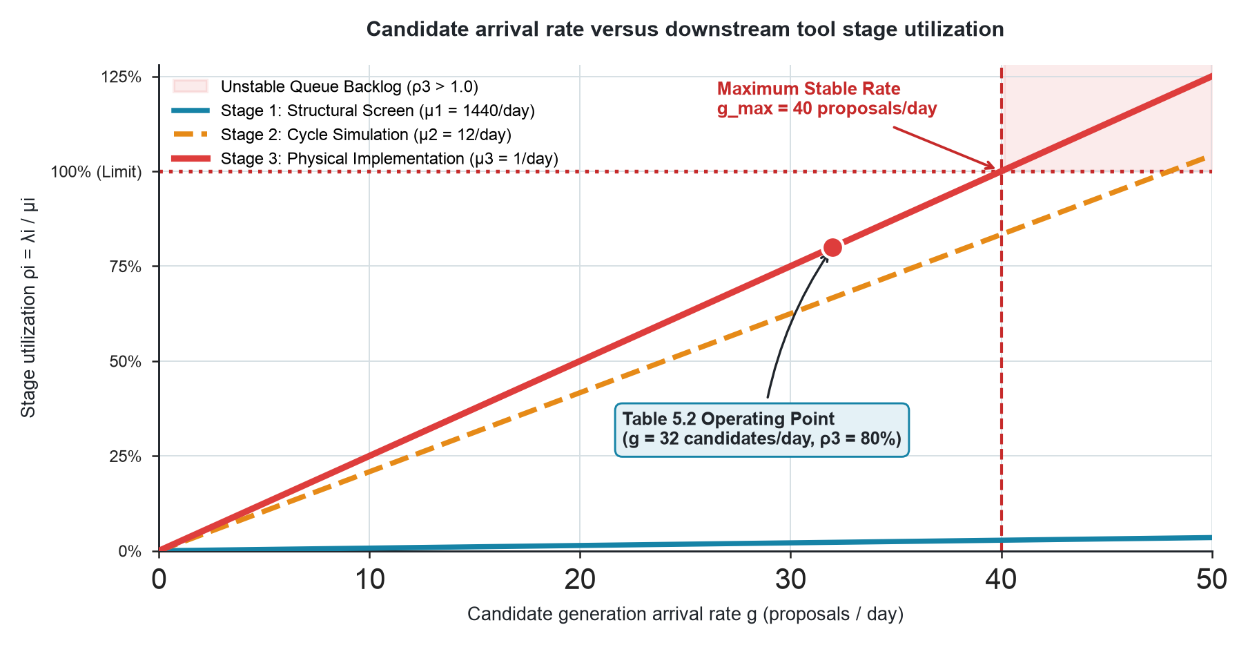
The structural screen receives all 32 candidates per day and operates at \(32/1{,}440\), or 2.2%, utilization. 8 candidates per day reach simulation, which operates at 66.7%. Only 0.8 candidates per day reach the implementation screen, which operates at 80%. Implementation is therefore our active capacity limit even though simulation handles more work. The expected finalist rate after all three stages is
\[ q = g \prod_i p_i. \tag{5.2}\]
For the illustrative values, this yields an expected finalist throughput in Equation 5.2 of 0.40 finalists per day. That product is a flow calculation, not the probability that a finalist is correct. It is also not our architecture-decision throughput. A supported decision may require several finalists, a matched baseline, additional checks, and architect review. Branching, return paths, correlated failures, variable service times, and shared licenses require a much richer model. Until we include design-team review capacity, this pre-review model cannot establish our total evaluation capacity or decision capacity.
Downstream tool capacity, not proposal rate, governs pipeline feasibility (Figure 5.3). The structural screen sits at near-zero utilization and cycle simulation scales moderately, but physical implementation screening climbs steeply because of its 24-hour execution latency. At the illustrative operating point of 32 candidates per day (Table 5.3), Stage 3 runs at 80 percent utilization (\(\rho_3 = 0.80\)), leaving 20 percent headroom for retries and tool licensing delays. As the arrival rate rises toward \(g_{\text{max}} = 40 \text{ proposals/day}\), Stage 3 reaches the queue stability limit (\(\rho_3 = 1.0\)); pushing generation past 40 candidates per day drives it into the unstable backlog region, where unverified candidates accumulate faster than signoff tools can evaluate them.
This simple calculation remains useful for method choice. Generation tends to increase \(g\). An early deterministic screen can reduce the load we pass forward. Prediction consumes qualification and later confirmation work while potentially reducing expensive evaluations. Optimization decides how we spend our available evaluation capacity. When our modeled tool stage is saturated, adding candidate production cannot remove the bottleneck. We face the same consequence if our separately assessed design-team review is saturated. We must reduce incoming work, reduce service time, add justified capacity, or change what needs the scarce check.
Recorded evaluation costs can guide our choice. A simulator result, warning, failed run, synthesis report, measurement, or expert review can reduce the uncertainty relevant to our decision. One synthesis run that distinguishes our two leading candidates may be worth more than another hundred proxy scores that merely preserve their ranking. We should ask which uncertainty the next evaluation can resolve, whether that result could change the candidate ranking or claim, and what the evaluation will ultimately cost. Raw run count is not our objective. A method-cost comparison that omits checking, review, qualification, confirmation, and the evaluations a search spends ends up pricing the component rather than the overall approach.
The value of each evaluation also depends heavily on what our environment records. Workload identity, candidate state, tool warnings, failure reasons, and evaluation conditions all make a result reusable. While Chapter 6 defines how our environment captures those returns, at this stage, we need to include them in our approach budget.
Recorded evaluation cost and the active-stage calculation supply the evidence we need for our limiting-work and saturated-checking tests above. If expensive evaluation is our active limit, a predictor earns a role only when screening saves more of that capacity than our qualification and confirmation consume.
5.3 Cost Models and Simulators
When an architectural design space expands into thousands of microarchitectural variations, subjecting every candidate to cycle-accurate simulation or physical synthesis quickly becomes impossible. In these high-dimensional regimes, surrogate cost models and predictive estimators allow us to trade absolute numerical accuracy for evaluation throughput. Predicting performance, power, congestion, or feasibility risks across candidate configurations enables us to screen vast search spaces long before committing scarce compute hours to detailed simulation flows. Architectural predictors are not a modern invention born of deep learning; our discipline relied on regression models and learned surrogates, including early neural predictors, to navigate complex design trade-offs long before large language models emerged (Ipek et al. 2006; B. C. Lee and Brooks 2006). Estimating the branch direction miss rate across complex instruction streams or evaluating NPU memory tiling factors across systolic dimensions requires extensive simulation. Fast regression or neural surrogates let us screen thousands of microarchitectural configurations before committing scarce simulation hours.
Ipek, Engin, Sally A. McKee, Rich Caruana, Bronis R. de Supinski, and Martin Schulz. 2006. “Efficiently Exploring Architectural Design Spaces via Predictive Modeling.” Proceedings of the 12th International Conference on Architectural Support for Programming Languages and Operating Systems, ASPLOS XII, 195–206. https://doi.org/10.1145/1168857.1168882.
Lee, Benjamin C., and David M. Brooks. 2006. “Accurate and Efficient Regression Modeling for Microarchitectural Performance and Power Prediction.” Proceedings of the 12th International Conference on Architectural Support for Programming Languages and Operating Systems, ASPLOS XII, 185–94. https://doi.org/10.1145/1168857.1168881.
Any predictor we build must estimate a consequence that our downstream decision actually consumes. We select one by matching each candidate model family’s strong fit against its main reason for rejection (Table 5.4), so that the technique we pick has mathematical assumptions that match our data representation, system constraints, and physical design space.
| Predictive technique | Strong fit | Main reason to reject it |
|---|---|---|
| Analytical or mechanistic cost model | Known relationships, limited data, and a need for inspectable assumptions. | The omitted interaction controls the decision. |
| Linear, polynomial, or regularized regression | Stable tabular features and a relationship that can be represented with modest complexity. | The response changes sharply or important structure is absent from the features. |
| Decision trees, random forests, and gradient-boosted trees | Tabular parameters, nonlinear interactions, and mixed feature types. | The method extrapolates into a design region unsupported by observations. |
| Gaussian process | Costly evaluations, moderate dimension, and a need to couple prediction with uncertainty-aware selection. | The space or dataset makes the surrogate costly or poorly matched. |
| Neural model | Large datasets from matching conditions and nonlinear behavior that simpler models do not capture. | Data coverage, latency, or confidentiality does not support training or use. |
| Sequence or transformer model | Programs, traces, reports, or time-dependent behavior whose order and long-range context matter. | The representation, dataset, or deployment budget cannot support the added flexibility. |
| Graph neural network | Netlists, dependency graphs, and other objects where connectivity carries the signal. | Node and edge features omit the property that controls the consequence. |
| Hybrid or simulator-corrected model | A useful analytical or low-fidelity model exists but has a repeatable residual error. | The correction data do not match the current tool, workload, or design region. |
| Transition or world model | Actions change later state and planning across several steps has value. | Independent candidate scoring or direct feedback is sufficient. |
Our choice of technique always depends on the relationship we need to model, the data we have to support it, and the constraints that might disqualify it. More flexible models do not automatically dominate simpler ones. We might find that a simple regression is the stronger choice when our data are scarce and the underlying relationship is stable. Conversely, a graph model justifies its complexity only when structural connectivity carries the exact information our decision requires.
Architecture world model: In this chapter, an architecture world model is a learned predictor of how represented design state, a permitted action, and stated conditions affect a later state or measured behavior. This is the chapter’s architecture-specific working definition, informed by the broader learned-world-model lineage (Ha and Schmidhuber 2018). It is one kind of predictive technique, not a fourth method family or one universal model of architecture.
Ha, David, and Jürgen Schmidhuber. 2018. “World Models.” arXiv Preprint arXiv:1803.10122, ahead of print. https://doi.org/10.48550/arXiv.1803.10122.
Transition model: A transition model predicts how selected design state or a decision-relevant consequence may change after a permitted action or sequence of actions under stated conditions.
Consider how we might tackle sequential macro placement. We feed our represented partial floorplan and a legal macro-location action into a transition predictor. We then perform a bounded rollout, which is a predicted action sequence limited in how many alternatives it explores and how many steps it looks ahead. Using this transition predictor, our planner compares these generated sequences and selects the single best first action. We only send that chosen action down our actual, declared placement tool path. Once the tool returns an observation, we qualify the result, update our represented state, and trigger replanning. Throughout this loop, we still rely on deterministic checks to exclude overlaps and blocked sites. The qualified placement and routing results then act as the high-fidelity observations we need to reliably assess congestion, timing, and routability.
We can draw a bounded precedent for this pattern from model-based policy optimization. When researchers tackled continuous-control tasks, they used short, model-generated rollouts branched from real observations to reduce accumulating model error, all while retaining the sample-efficiency benefits of a learned dynamics model (Janner et al. 2019). However, that result does not hand us a ready-made rollout horizon, state representation, or dynamics model for architecture. Our placement, compilation, and microarchitecture tools all exhibit vastly different state transitions and failure conditions. Therefore, we must qualify our predictor against our own tool returns, ensuring we send every selected action or surviving candidate back through a declared, high-fidelity tool path before we trust it in a final design decision.
Janner, Michael, Justin Fu, Marvin Zhang, and Sergey Levine. 2019. “When to Trust Your Model: Model-Based Policy Optimization.” Advances in Neural Information Processing Systems 32. https://papers.nips.cc/paper/2019/hash/5faf461eff3099671ad63c6f3f094f7f-Abstract.html.
We can see the heavy cost of this composition when we contrast it with two simpler alternatives. If we use independent static scoring, we simply estimate each complete candidate without predicting how one action changes our later choices. If we use a model-free policy, we map our observed state directly to an action, skipping explicit predicted rollouts entirely. Our world model only earns its expensive predictor and planner when the action horizon is long enough for sequence effects to matter, and when our bounded rollouts save enough real tool calls to offset the overhead of model fitting, accumulated prediction error, and intermediate state checks. If we have cheap tool feedback, a short horizon, rapidly compounding rollout errors, or a checking cost that rivals direct execution, we should abandon the world model in favor of static scoring, a model-free policy, or simply using the tool directly.
Different architecture jobs will naturally demand different state and consequence models. We do not need our compiler-tuning model, our placement-transition model, and our cache-performance model to share a single, unified state or output representation. Throughout this process, our current state must remain the represented design state we defined in Chapter 4, never an unconfirmed prediction. A world model can guide our search without becoming authoritative project state, so we preserve separate execution paths for model prediction and direct tool observation under recorded conditions (Figure 5.4).
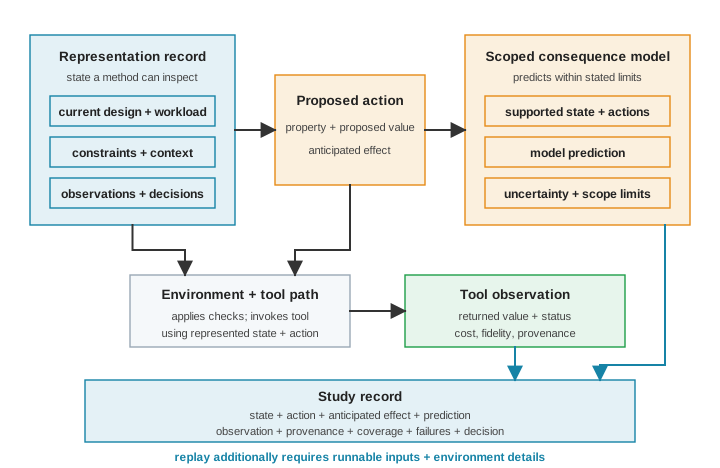
Prediction and direct tool observation remain distinct records (Figure 5.4). The same represented state and proposed action feed a scoped consequence model, which incorporates a transition model when state dynamics matter, and a declared tool or simulator path. Both returns land in a versioned study record. The consequence model estimates behavior within qualified bounds. The direct tool path supplies a reference observation under its own model, configuration, and fidelity. Qualified agreement lets us continue using the model within its stated support region, but it does not make either return authoritative outside its declared conditions.
5.4 Predictor Support Boundaries
A predictive surrogate is only as reliable as the empirical support underlying its training data. The moment an architectural optimizer steers a search into uncharacterized design regions, unexpected workload mixes, or modified process corners, surrogate predictions can fail silently. In hardware design, a surrogate that reports low average error across a global dataset can still misrank top candidates at a critical decision boundary or hallucinate feasibility under strict power limits. Qualification requires us to audit predictor support boundaries against high-fidelity tool baselines before trusting surrogate predictions to filter real candidates. When we deploy a screening surrogate, it must preserve the correct ordering near our decision boundaries, where rank correlation and top-k recall1 matter much more than a model’s global average error. However, we still care about point accuracy whenever a hard limit, such as an area constraint or maximum access time, dictates a design’s feasibility. Our assessment criteria must align directly with the specific decisions, candidate regions, workloads, and thresholds at play, rather than collapsing everything into a single aggregate score.
1 Top-k recall: The fraction of the measured best k candidates that also appear in our predictor’s top k. It asks whether our screen successfully retained the designs worth evaluating, which is fundamentally different from asking whether all predicted values were numerically accurate. For instance, Ansor, a tensor-program autotuner, uses this measure to determine whether its cost model successfully preserves promising tensor programs for our subsequent evaluation (Zheng et al. 2020).
Zheng, Lianmin, Chengfan Jia, Minmin Sun, et al. 2020. “Ansor: Generating High-Performance Tensor Programs for Deep Learning.” 14th USENIX Symposium on Operating Systems Design and Implementation (OSDI 20), November, 863–79. https://www.usenix.org/conference/osdi20/presentation/zheng.
Before we let a cheap predictor gate which candidates reach our expensive tools, we need to reserve a dedicated check batch sampled directly from the candidate and condition regions where that screen will actually operate. We cannot use this batch to fit or tune our predictor. Instead, we must send these test cases through both paths. Applying decision-aligned ranking measures, such as top-k recall, we can determine exactly how many candidates need to survive our screen to ensure we hold onto the designs truly worth measuring. If we see weak recall, we have to either expand our survivor set or abandon the screen altogether. These check runs consume the same evaluation budget our predictor was supposed to save.
When we qualify a predictor, we are comparing our cheap proxy against a stronger reference baseline across the specific region where we intend to deploy it. Depending on our goal, the relevant comparison might focus on numerical error near a critical threshold, ranking agreement for a screening pass, or interval coverage to back up an uncertainty claim. In contrast, calibration represents the narrower task of establishing a declared numerical or probabilistic mapping, whether that takes the form of an interval, a threshold, or a specific confidence guarantee.
Through qualification, we determine whether a given predictor is actually suitable for its planned role and whether the necessary reference runs fit within our overall study budget. Once our proxy returns a value, we then rely on Section 7.6 to determine exactly which architectural conclusions that specific value can safely support.
Our predictions become dangerous the moment an optimizer pushes them into a design or workload region that looks nothing like our training and qualification data. We also know that learned uncertainty estimates can fail drastically once the underlying data-generating conditions shift (Ovadia et al. 2019). When working with architecture predictors, introducing a new workload mix, upgrading a tool version, shifting process conditions, or exploring an unfamiliar design region can immediately invalidate both our core estimates and their associated uncertainty bounds. Consequently, a wide or narrow interval cannot by itself diagnose this kind of fundamental mismatch.
Ovadia, Yaniv, Emily Fertig, Jie Ren, et al. 2019. “Can You Trust Your Model’s Uncertainty? Evaluating Predictive Uncertainty Under Dataset Shift.” Advances in Neural Information Processing Systems 32: 13991–4002. https://proceedings.neurips.cc/paper_files/paper/2019/hash/8558cb408c1d76621371888657d2eb1d-Abstract.html.
2 Conformal prediction: A statistical technique that produces prediction sets or intervals from a model, providing finite-sample coverage guarantees under an exchangeability assumption (Lei et al. 2018; Angelopoulos and Bates 2021). In our context, we might use a calibrated interval to prune, defer, or escalate a candidate, but we should never use it alone to authorize a final design decision.
When we rely on learned world models, we introduce a sequence-specific flavor to this same problem. An error that seems acceptable after a single permitted action can rapidly accumulate across a longer sequence, eventually driving our predicted state far outside its qualified region. Therefore, we must explicitly qualify our maximum sequence length and compare any predicted intermediate states against real tool observations before we trust them to guide our subsequent actions. We can use conformal prediction2 to attach a calibrated interval \(\hat{C}(x)\) to a surrogate, expressed as
\[\hat{C}(x) = [f(x) - q_{1-\alpha}, \, f(x) + q_{1-\alpha}]\]
where \(q_{1-\alpha}\) represents the \((1-\alpha)(1 + 1/n)\) empirical quantile of calibration nonconformity scores \(|y_i - f(x_i)|\), provided we rely on an exchangeability assumption3 and select a valid nonconformity score4 (Lei et al. 2018; Angelopoulos and Bates 2021). Imagine driving a vehicle equipped with an automated navigation system calibrated for smooth highway asphalt. As long as the vehicle stays on the highway (the calibrated support region), its predicted stopping distances hold true. However, if an optimizer steers the vehicle off-road into unmapped mud (a distribution shift where \(P_{\text{test}}(X,Y) \neq P_{\text{train}}(X,Y)\)), the empirical coverage \(\mathbb{P}(Y \in \hat{C}(X))\) collapses silently below \(1-\alpha\) because the underlying friction mechanics have changed (Tibshirani et al. 2019). In architectural surrogate modeling, conformal intervals provide margins of safety only within the boundaries where exchangeability holds true, and the moment our workload or design corner shifts, those mathematical guarantees vanish.
3 Exchangeability: A statistical property where the joint distribution of a sequence of random variables remains invariant to their permutation, serving as a weaker assumption than being independent and identically distributed (i.i.d.) (Lei et al. 2018). Because our architecture workloads, tools, and process corners frequently violate this property, we must strictly audit, rather than blindly trust, any conformal interval we produce.
4 Nonconformity score: A function we use to measure how poorly our fitted model agrees with an observed calibration case. In split-conformal regression, we often define this as the absolute residual between our prediction and the observation. As shown in our fixed-width construction here, we choose a specific quantile of those calibration scores to lock in our interval width (Lei et al. 2018).
Tibshirani, Ryan J., Rina Foygel Barber, Emmanuel Candes, and Aaditya Ramdas. 2019. “Conformal Prediction Under Covariate Shift.” Advances in Neural Information Processing Systems (NeurIPS) 32: 2530–40.
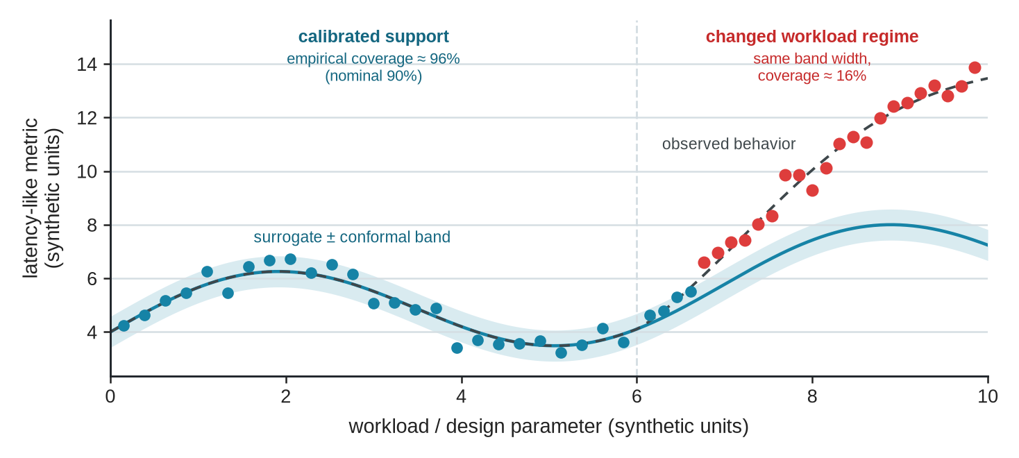
Nominal marginal coverage from one design region cannot justify a screening pass once the workload distribution shifts (Figure 5.5). A fixed-width split-conformal band around a surrogate holds its nominal 90 percent coverage inside the calibrated support regime (\(x \le 6.0\)), but once the workload changes (\(x > 6.0\)) the true latency drifts upward while the interval stays fixed, so coverage collapses exactly where exchangeability fails.
We can only justify predictor-based screening while its calibrated coverage survives under the exact conditions where it operates. Inside the calibrated support the empirical coverage stays near nominal, and it collapses once the workload response changes while the interval remains unchanged (Figure 5.5). This synthetic construction does not estimate the true failure rate of a real architecture predictor; what it fixes is the rule that we can never carry nominal marginal coverage from one support region into a screening pass once the relevant workload or design response shifts.
Before deploying any predictor, we must define a strict audit window. We can frame this as a fixed number of screened candidates, an elapsed interval, or a named workload and design batch where we pair our predictions directly against reference runs. We also need to state how often this check repeats and which recall, coverage, or threshold-error conditions will force us to halt our predictor-based work. Our synthetic illustration above does not offer a universal threshold for this. Instead, whenever our returned comparison crosses our own declared fail condition, we must immediately stop using the predictor for screening and hand the failing comparison, our current support claim, and whatever remains of our budget over to Chapter 7, which will then determine our next best action.
We must halt a predictor whenever we can no longer qualify its planned use, when our candidate escapes its stated support region, when the error grows too large to support our decision, or when direct evaluation becomes cheaper than maintaining the model itself. Because our predictor merely estimates a result, rather than fully replacing the robust tool or measurement our study originally requested, we must ensure our planned downstream checks remain visible and consistently enforced.
Our predictions can only estimate consequences for candidates that exist within our defined input space. Whenever a required artifact or candidate is missing, our limiting work shifts away from merely estimating an existing option; instead, we must pivot to physically constructing a new option that our later checks can properly evaluate.
5.5 Synthesizing Candidate Architecture Artifacts
Architectural exploration often stalls not from a lack of evaluation capacity, but from the absence of a candidate artifact. When we need an unwritten RTL module, a specialized compiler schedule, a custom testbench, or a novel floorplan topology, generative techniques allow us to synthesize structured hardware specifications directly from abstract requirements. Yet, candidate generation introduces an architectural trade-off, because every newly synthesized artifact shifts the engineering burden directly onto our downstream verification tools. We must never treat generation as an automatic default when candidates already exist or when parameterized templates and conventional compiler passes can construct the required artifact deterministically.
The nature of our artifact dictates which generative technique becomes plausible. Templates, grammars, rules, program synthesis, compiler passes, and parameterized generators naturally fit precisely structured artifacts; Halide’s separation of algorithm from schedule is the canonical compiler-side example (Ragan-Kelley et al. 2018). An autoregressive code model constructs a sequence one token at a time from the preceding tokens, an approach Codex, an autoregressive code-generation model, demonstrated for general-purpose software and Python program generation (M. Chen et al. 2021). When we shift to RTL generation, we need hardware-specific evidence (Liu, Ene, et al. 2023; Thakur et al. 2023). We evaluate the functional correctness of generated Verilog using benchmarks like VerilogEval, an evaluation benchmark for Verilog code generation, with an RTL testbench, whereas RTLLM, an LLM evaluation benchmark for hardware design, incorporates simulation and post-synthesis area, delay, and power metrics (Liu, Pinckney, et al. 2023; Lu et al. 2024). Neither benchmark establishes full signoff readiness or complete test generation for our designs. We can apply constrained decoding to block a next token when it would violate an encoded grammar or schema, which helps us reduce syntactically invalid work long before compilation (Willard and Louf 2023; Geng et al. 2023). We might also use retrieval to feed current project documents or examples into these techniques, though we must recognize retrieval as a supporting capability rather than a standalone generation family.
Ragan-Kelley, Jonathan, Andrew Adams, Dillon Sharlet, et al. 2018. “Halide: Decoupling Algorithms from Schedules for High-Performance Image Processing.” Communications of the ACM 61 (1): 106–15. https://doi.org/10.1145/3150211.
Chen, Mark, Jerry Tworek, Heewoo Jun, et al. 2021. “Evaluating Large Language Models Trained on Code.” arXiv Preprint arXiv:2107.03374, ahead of print. https://doi.org/10.48550/arXiv.2107.03374.
Liu, Mingjie, Teodor-Dumitru Ene, Robert Kirby, et al. 2023. ChipNeMo: Domain-Adapted LLMs for Chip Design. arXiv preprint arXiv:2311.00176. https://arxiv.org/abs/2311.00176.
Thakur, Shailja, Baleegh Ahmad, Hammond Pearce, et al. 2023. “VeriGen: A Large Language Model for Verilog Code Generation.” arXiv Preprint arXiv:2308.00708, ahead of print. https://doi.org/10.48550/arXiv.2308.00708.
Before we adopt retrieval-supported generation, fine-tuning, or any other method leveraging external or project material, our study must answer two independent questions. First, which sources can we use for training or retrieval, and what source links, licenses, attribution, and transformation history will remain available so we can properly assess our generated artifact’s provenance? We consider this the inbound question. If we use a model trained on code whose license terms propagate to derived work, it can reproduce enough of that code to prevent our generated RTL from clearing legal review. Second, which of our proprietary prompts, constraints, RTL, reports, and retrieved passages may safely leave our authorized project boundary, and through which execution and egress routes? We call this the outbound question, as it centers on our proprietary constraints reaching a third-party endpoint. Having permission to use an inbound source does not authorize us to disclose our current project’s material externally. Conversely, keeping our execution entirely local does not automatically establish acceptable inbound provenance for the generated output. If we cannot satisfy either condition, the technique ceases to be a usable path for our study.
Our graph and spatial artifacts demand construction methods capable of preserving very different structural properties. We apply graph-generative methods to objects where the nodes, edges, and connectivity carry the core design meaning. When we turn to diffusion-based spatial generators, we start with a noisy proposal and iteratively refine it, an approach that fits our placement and floorplan construction tasks well (V. Lee et al. 2025).
Lee, Vint, Minh Nguyen, Leena Elzeiny, Chun Deng, Pieter Abbeel, and John Wawrzynek. 2025. “Chip Placement with Diffusion Models.” Proceedings of the 42nd International Conference on Machine Learning, Proceedings of machine learning research, vol. 267: 33499–514. https://proceedings.mlr.press/v267/lee25y.html.
Because different artifacts expose distinct structures, our construction methods must enforce different constraints. Each candidate generation path carries a verification bound it can honor and one it cannot (Table 5.5): constrained decoding or spatial priors can enforce syntax and boundary geometry during synthesis, but property-specific simulation, timing analysis, and physical signoff remain mandatory whatever the artifact.
| Artifact or problem | Likely construction path | What the path can enforce or use | External check still required |
|---|---|---|---|
| Precisely structured configuration or program | Template, grammar-guided generator, solver, compiler pass, or program synthesis | Encoded syntax, types, and stated constraints | Intended semantics and implementation behavior |
| General-purpose software, script, or compiler code | Autoregressive code model or LLM, optionally with constrained decoding | Supplied context and encoded token or schema restrictions | Execution semantics, target behavior, and other artifact-specific properties |
| RTL | Autoregressive code model or LLM evaluated with an RTL-specific benchmark (Liu, Pinckney, et al. 2023; Lu et al. 2024) | Supplied design context and encoded token, grammar, or schema restrictions | Elaboration, CDC linting, reset synchronization, simulation, formal properties via SVA/BMC, synthesis in Yosys, static timing analysis in OpenSTA, power intent via UPF, and physical signoff checks required by the project |
| Project-specific text or code | Retrieval-supported generation | Current retrieved documents and examples, subject to their provenance and coverage | Source consistency and the checks required by the generated artifact |
| Netlist or connectivity object | Graph-generative or graph-conditioned method | Represented nodes, edges, and graph constraints | Electrical, functional, timing, and physical properties |
| Placement or floorplan | Diffusion or another spatial generator | Spatial proposal distribution, fixed block geometry, and encoded placement constraints | Legalization, routing, timing, power, and manufacturability |
| Mixed hard and learned constraints | Learned proposal followed by a solver, compiler, deterministic builder, or repair step | Hard constraints encoded by the conventional component and patterns learned from data from matching conditions | Every relevant property not established by the encoded constraints |
How we handle constraints determines how much flawed work reaches our downstream tools. While constrained decoding can guarantee membership in an encoded grammar (Willard and Louf 2023; Geng et al. 2023), it cannot establish elaboration, functional correctness, routability, timing, or power for our designs. A spatial generator faces the same boundary. It can propose a layout, but we rely on later tools to determine which of our declared physical conditions that layout actually satisfies. Neurosymbolic AI addresses this exact boundary by coupling probabilistic neural generators directly with symbolic verifiers such as AST type checkers, SAT or SMT solvers, and static compiler passes. The neural component proposes broad candidate structures while the symbolic engine enforces structural and semantic correctness before candidates hit heavy evaluation tools. Even within a neurosymbolic flow, our final artifact still requires its property-specific checks.
Willard, Brandon T., and Rémi Louf. 2023. Efficient Guided Generation for Large Language Models. https://doi.org/10.48550/arXiv.2307.09702.
Geng, Saibo, Martin Josifoski, Maxime Peyrard, and Robert West. 2023. “Grammar-Constrained Decoding for Structured NLP Tasks Without Finetuning.” Proceedings of the 2023 Conference on Empirical Methods in Natural Language Processing (EMNLP) (Singapore), 10932–52. https://doi.org/10.18653/v1/2023.emnlp-main.674.
Our generator therefore requires a clearly scoped input, legal actions, and inexpensive early checks. A syntactically valid RTL fragment may still fail our functional simulation in Verilator, an open-source SystemVerilog simulator, or logic synthesis in Yosys, an open-source RTL synthesis suite, before even reaching physical layout. A generated LLVM compiler pass pipeline or NPU dataflow tile schedule might likewise be perfectly legal while creating unacceptable data movement or buffering overhead. We find generation useful only when an early check can reject poor proposals before they consume our scarce tool resources and review capacity. Whenever our generated artifact is executable or synthesizable, we must establish its functional correctness before we compare its performance.
A generated checker does not automatically provide independent verification. If our generator emits both the RTL and its testbench, it may repeat the same misinterpreted requirement across both artifacts. While the checker can still expose simple errors, achieving true independence requires us to use a sufficiently different oracle, tool, implementation, or reviewer, along with an explicit account of whichever assumptions remain shared across our flow.
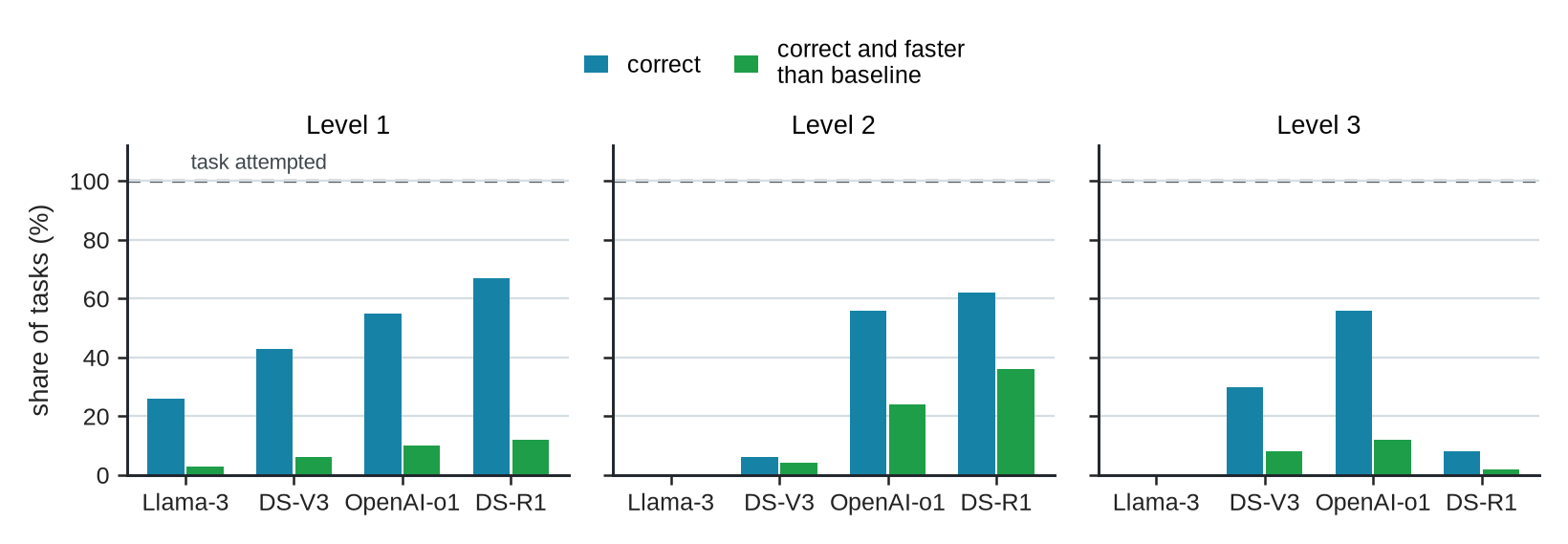
We should stop generation when our study secures enough useful alternatives, when our checking or review bandwidth becomes the new bottleneck, or when the generator repeatedly wanders outside our represented action space. It must never widen that space silently. High-Level Synthesis (HLS, which compiles algorithmic C/C++ specifications into register-transfer level hardware descriptions) C/C++ pragma design space exploration (DSE, which systematically evaluates compiler annotations to trade off execution throughput against physical hardware area) makes this separation visible, because hardware synthesis flows depend entirely on target-specific C/C++ annotations that must be both syntactically legal and timing-feasible. In an HLS pragma DSE workflow, a generator or optimizer inserts loop unrolling (#pragma HLS UNROLL), pipelining (#pragma HLS PIPELINE), and array partitioning (#pragma HLS ARRAY_PARTITION) pragmas into C/C++ compute kernels. An execution harness compiles each candidate via Vitis HLS or Vivado HLS (Xilinx high-level synthesis tools), verifies functional correctness with C/RTL co-simulation, and evaluates target latency, initiation interval, and FPGA/ASIC resource utilization, specifically Look-Up Tables (LUTs), Digital Signal Processors (DSPs), and Block RAMs (BRAMs). Software kernel generation benchmarks such as KernelBench, a GPU code generation benchmark, exhibit a parallel candidate funnel for GPU code generation, where language models propose kernels written in CUDA, NVIDIA’s parallel computing platform, evaluated against a baseline in PyTorch, an open-source machine learning framework (Ouyang et al. 2025).
Candidate retention drops steeply at each stage, so code syntax, functional correctness, and performance are distinct checks (Figure 5.6). Across difficulty levels 1, 2, and 3 on an NVIDIA L40S GPU, four language models (Llama-3.1-70B, DeepSeek V3, OpenAI o1, and DeepSeek R1) attempt every task, but only 0 to 67 percent of their one-shot kernels pass functional correctness, and just 0 to 36 percent are both correct and faster than the PyTorch Eager baseline. Attempted is not correct, and correct is not fast.
Ouyang, Anne, Simon Guo, Simran Arora, et al. 2025. “KernelBench: Can LLMs Write Efficient GPU Kernels?” arXiv Preprint arXiv:2502.10517, ahead of print. https://doi.org/10.48550/arXiv.2502.10517.
The measured KernelBench funnel narrows sharply as it moves from attempted candidates to functionally correct implementations and finally to kernels that outperform their baseline. A prospective HLS pragma DSE study would narrow the same way, with C/RTL co-simulation and synthesis reports deciding which candidates meet target latency, initiation interval, and area budgets. As architects, we cannot infer hardware quality from apparent C/C++ code fluency or from an overall model ranking. Instead, the generator proposes the pragma-annotated C/C++ candidate, our HLS compiler and C/RTL co-simulation harness dictates its functional correctness, and our physical synthesis flow determines whether the candidate achieves superior performance, power, and area (PPA) trade-offs under tested target conditions.
When we build a reusable HLS pragma DSE evaluation, we must record the target FPGA or ASIC library, our correctness oracle (C-simulation and C/RTL co-simulation), numerical tolerances, clock targets, resource constraints, and explicit rejection rules for fast but timing-violated designs. If proposals arrive faster than Vitis HLS or Vivado HLS synthesis runs can evaluate them, generating more candidates lengthens our backlog without accelerating design discovery.
To construct a fair method comparison, we must ask how the missing artifact is constructed, not just whether the final output beats an unoptimized C/C++ baseline. While an unpragma’d C baseline provides a reference, it does not represent our strongest conventional construction path. A compiler autotuner (such as AutoTVM or Vitis HLS Tcl search scripts) or a domain-specific solver can often discover optimal pragma allocations without relying on LLM code generation.
A fair study requires us to give the learned and conventional construction paths the exact same task specification, target device, numerical tolerance, permitted pragma transformations, online context, allowed tool feedback, and computational budget. We must force both paths to pass the same compilation, C/RTL co-simulation, and synthesis checks before any PPA metrics count. We must also acknowledge that true costs include failed synthesis runs, C/RTL co-simulations, setup overhead, and expert review time. Our comparison can then properly ask whether learned generation produces a correct and faster design, reaches a comparable result with less total work, or successfully supplies an artifact that our conventional path cannot produce within budget. While KernelBench demonstrates the output checks and candidate funnel for GPU software kernels, it does not by itself settle this hardware synthesis comparison for us.
We must fix these conditions firmly before any execution begins (Table 5.6). For one C/C++ compute kernel under HLS pragma DSE, we pin the shapes, data types, target FPGA/ASIC libraries, and synthesis engines before choosing either constructor, so that conventional autotuners and code-generation models compete under identical evaluation rules over the same tools, checks, and matched resources.
| Aspect | Prospective matched-construction comparison |
|---|---|
| Artifact and semantics | Pin one executable C/C++ compute kernel (such as 2D convolution or matrix multiplication), target FPGA/ASIC library, target clock, numerical tolerance, and HLS tool version before selecting either constructor. |
| Construction arms | Predeclare one strongest practical conventional HLS autotuner (such as a Tcl pragma search or solver-backed DSE), and one code-generating model or pragma optimizer. Both receive the same compute kernel and permitted tool returns. |
| Shared tools and checks | Both paths use the same Vitis HLS flow, C-simulation, C/RTL co-simulation harness, logic synthesis, and timing signoff. Noncompiling or functionally incorrect candidates cannot enter the PPA comparison. |
| Matched resources | Pin the online context, wall-clock limit, synthesis execution allowance, and expert setup allowance. Declare arm-specific pretrained models, HLS libraries, pragma templates, and prebuilt assets. |
| Recorded result | Retain attempted artifacts, synthesis failures, latency/II metrics, resource utilization (LUTs, DSPs, BRAMs), tool cost, elapsed time, and expert work. Compare total work only after an artifact passes shared checks, and leave the result unresolved if neither path succeeds within budget. |
Our shared compiler and correctness harness must first determine whether either path produced a usable kernel. Performance separates our accepted artifacts only after they pass that check. If our learned kernel runs faster but demands substantially more construction and review effort, we must recognize that as a tradeoff, rather than an automatic win.
We can transfer this same test to RTL. We should compare a learned RTL generator directly against a serious parameterized generator, a template, a high-level synthesis path, or a solver-backed construction method under the identical interface contract, allowed changes, testbench, implementation tools, and engineering budget. In many cases, we may find the result favors our conventional path.
Chip-Chat, an interactive hardware design study, brings this same role separation directly into RTL design (Blocklove et al. 2023). In this project, a language model drafted Verilog for a small 8-bit processor that successfully reached tapeout only after a human guided it through many revisions. Open-source simulation and synthesis tools returned strict errors that could reject or redirect drafts, while the human designer ultimately decided when a candidate was ready to advance. This example shows us why we can never separate our generation cost from our checking cost. Whether we find that total cost acceptable depends heavily on the artifact in question, our tool latency, and our available review capacity.
Blocklove, Jason, Siddharth Garg, Ramesh Karri, and Hammond Pearce. 2023. “Chip-Chat: Challenges and Opportunities in Conversational Hardware Design.” 2023 ACM/IEEE 5th Workshop on Machine Learning for CAD (MLCAD), 1–6. https://doi.org/10.1109/MLCAD58807.2023.10299874.
While our construction methods can remove a shortage of candidates, they often end up creating a new bottleneck. Whenever candidates arrive faster than our scarce tool runs can possibly evaluate them, our selection process, rather than the construction itself, becomes our limiting work.
5.6 Search Tactics and Budget Allocation
When an architectural search space expands beyond what brute-force enumeration or exhaustive simulation can evaluate, optimization algorithms become necessary for rationing our evaluation budget. Every automated search procedure faces a dilemma over whether to exploit known, high-performing regions of the design space or to explore uncharacterized regions where superior configurations might lie. Choosing the right search tactic requires matching the mathematical structure of our parameter space (whether continuous, discrete, or mixed-integer) to the physical cost of acquiring candidate feedback. A search procedure that excels at continuous transistor sizing can stall when applied to discrete cache topologies or sequential macro placement.
Because an optimizer can only improve based on the feedback it receives from our evaluation path, we must give every returned metric an explicit meaning. We have to treat known legality and tool-discovered feasibility differently. When we know about constraints ahead of time, such as an enumerated cache capacity or a nonoverlap rule, we should encode them directly into our candidate construction or action operators if possible. Alternatively, we can apply them as a deterministic rejection or projection step before we waste a scarce evaluation. In contrast, downstream steps like placement, routing, timing, simulation, or implementation might only expose additional limits after our tools actually run. Even a valid, completed result only proves a candidate is feasible or infeasible under our specific choice of tool, settings, effort, resource budget, and stopping condition. If we halt a run at a declared time or resource limit, it returns an incomplete or timeout signal. At that point, the completion time is “right-censored,” which is the statistical term for an event that we only know occurs sometime after our observation window closes (Klein and Moeschberger 2003).
Klein, John P., and Melvin L. Moeschberger. 2003. Survival Analysis: Techniques for Censored and Truncated Data. 2nd ed. Statistics for Biology and Health. Springer. https://doi.org/10.1007/b97377.
A timeout gives us no objective value unless our optimization formulation explicitly models censored outcomes. Even with a formal censoring model in place, a timeout only tells us that the run exceeded our limit, rather than giving us its exact completion time, and it leaves all other objectives unobserved. If a run instead ends in a crash, leaves a stale workspace, or fails to produce a required artifact, it yields no objective value at all. We must record these as invalid runs or infrastructure failures. If we repeatedly encounter feasibility failures, we might want to switch to constrained optimization or build a separate feasibility predictor, but the declared design tools still provide the reference observations for those scoped conditions.
We also have to watch out for bias when we select the best among many surrogate-scored candidates. Even if our surrogate’s prediction errors average perfectly to zero, the act of selecting a winner inherently favors candidates that enjoyed optimistically large errors. As a result, our winner’s predicted gain will often exceed the gain we actually observe later, and this gap tends to widen as we increase the size of our candidate pool or the noise in our scores. We call this the optimizer’s curse (Smith and Winkler 2006). To protect ourselves, we need to preserve the originally predicted score, reserve an independent confirmation run tailored to the variability of our decision, and honestly report any shrinkage rather than dressing up a selected prediction as our final result.
When we work within a fixed search space, we use “exploration” and “exploitation” to describe where our optimizer chooses to spend its next evaluation. Exploitation means we sample regions where the results already look promising. Exploration means we sample the less-understood corners of that same declared space. Importantly, neither strategy actually widens our boundaries. If we want to evaluate an entirely new topology, dataflow, ISA extension, or cache policy, we have to reopen our study formulation and change our representation.
To guide this process, we rely on an acquisition function that balances surrogate predictions with estimated uncertainty to select our next evaluation point (Figure 5.7).
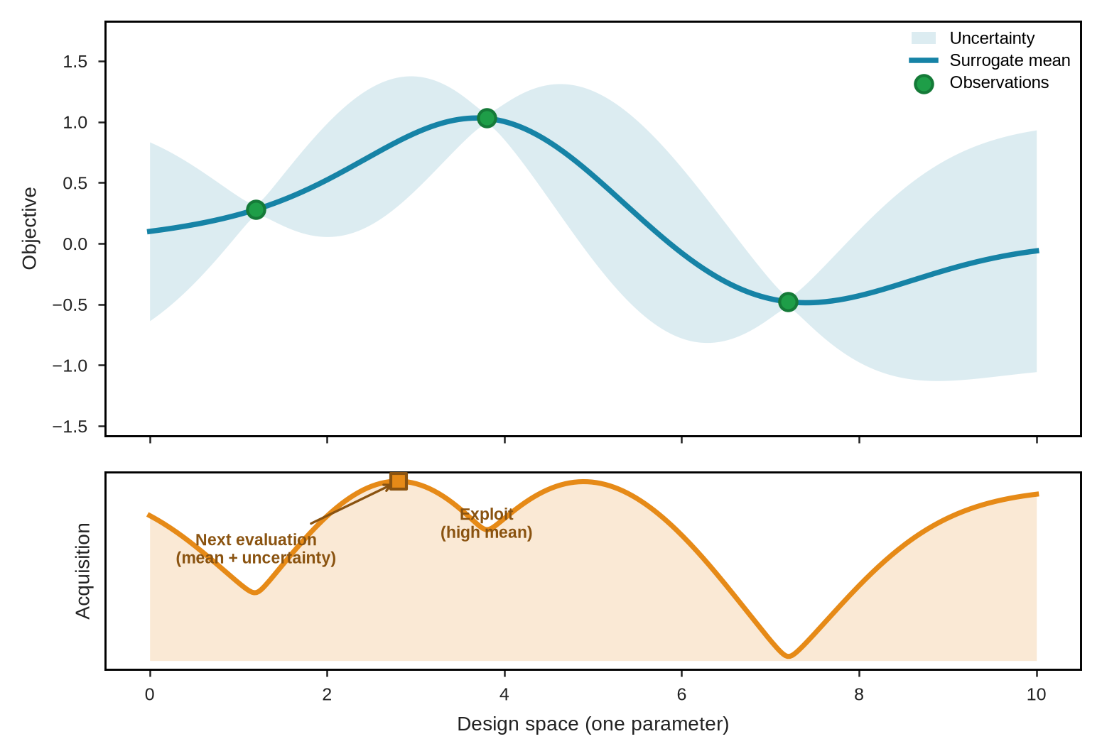
Bayesian optimization trades exploitation of high-mean regions against exploration of high-uncertainty ones across a single-parameter space (Figure 5.7). A Gaussian process surrogate mean carries three observations under a \(\pm 1 \sigma\) uncertainty band that widens where we have not sampled, and the upper-confidence-bound acquisition function \(\mu(x) + \kappa \cdot \sigma(x)\) combines the two. An exploitation peak sits near high predicted performance (\(x \approx 3.8\)), but the global acquisition maximum falls just beside it at \(x \approx 2.8\), where a still-favorable mean meets the uncertainty that grows between our observations. That is where we send the next physical tool evaluation, rather than at the sampled point itself. Keeping surrogate prediction separate from acquisition selection lets us probe high-uncertainty regions without mistaking early predictions for final observations.
The shaded band in the figure represents only the model’s uncertainty arising from sparse observations; it does not capture every underlying source of run-to-run variability. Because our surrogate and our acquisition rule perform different jobs, we must ensure they remain separately inspectable, even if a vendor packages them together in a single implementation. Our optimizer does not define the architectural question, nor does it authorize the final result. It merely selects candidates for evaluation within the action space, objective, constraints, and stopping conditions we declare, while respecting the limits we set on the number, latency, cost, and fidelity of those evaluations.
When we use multi-fidelity Bayesian optimization,5 we extend this choice to also select the evaluation fidelity (Kandasamy et al. 2017). To ensure reproducibility, our execution request should ask the environment to retain our acquisition rule, fidelity choices, assumptions, returned results, rejected alternatives, and any escalation thresholds we applied.
5 Multi-fidelity Bayesian optimization: Jointly chooses which design we should evaluate and at which fidelity level, trading expected information gain against cost (Kandasamy et al. 2017). The selection policy itself does not decide what claims our distinct feedback levels can ultimately establish.
Kandasamy, Kirthevasan, Gautam Dasarathy, Jeff Schneider, and Barnabás Póczos. 2017. “Multi-Fidelity Bayesian Optimisation with Continuous Approximations.” Proceedings of the 34th International Conference on Machine Learning (ICML), Proceedings of machine learning research, vol. 70: 1799–808. https://proceedings.mlr.press/v70/kandasamy17a.html.
5.7 Algorithmic Search Tactics and Heuristics
Once we establish our evaluation budget and acquisition framework, selecting an effective search tactic requires matching the optimization algorithm to the geometry and structure of our design space. Choosing an algorithm by reputation without examining its assumptions often creates unnecessary sample complexity or search stagnation. Small, bounded spaces usually make enumeration or deterministic domain heuristics strong starting points. Bayesian optimization can be attractive when evaluations are expensive and a useful surrogate can be fit over the active region. Evolutionary search, local heuristics, constraint solving, and other procedures may fit large discrete spaces, depending on representation and feedback cost. Reinforcement learning becomes plausible only when actions create meaningful sequential state and repeated interaction is affordable. These are starting hypotheses, not assignments determined by dimensionality alone.
If our legal space contains many declared parameters, we can often benefit from running a screening experiment before we launch our main search. In a screen, we deliberately vary a limited set of factor combinations to estimate which main parameters actually move our decision-relevant metrics enough to justify further evaluation (Plackett and Burman 1946). However, we must treat this as an optional tool rather than a required stage. If our system has strong interactions or discrete topology changes, or if we build our screen on a weak proxy, the resulting parameter rankings can be deeply misleading. Just because a parameter looks unimportant inside our narrowly screened region does not prove it will remain irrelevant everywhere else.
Plackett, Robin L., and J. Peter Burman. 1946. “The Design of Optimum Multifactorial Experiments.” Biometrika 33 (4): 305–25.
Whenever our objectives and constraints admit a useful algebraic formulation, we can use mathematical programming or constraint solving to exploit that structure directly. This direct approach is almost always preferable to paying the overhead for a learned search procedure. However, a solver only establishes exactly what we put into its formulation. Because of this, if we omit downstream physical or software effects, we still need to catch them with relevant checks later.
Reinforcement learning serves a different purpose. We can defend its use most easily when our problem is genuinely sequential. In these cases, an action changes the state, our later choices depend heavily on our earlier ones, and we can afford repeated interactions with the environment. Macro placement offers an example of this formulation. When a placement policy chooses one macro location at a time, the updated partial floorplan becomes the state for our next choice.
But even a strong sequential fit is not enough if interacting with the environment is too expensive. We have to count our training runs, tuning cycles, random seeds, retries, and final policy evaluations at the fidelities they consume. If we cannot amortize high-fidelity simulation, synthesis, or placement calls across related tasks, and we cannot replace them during learning with a qualified lower-fidelity path, then reinforcement learning makes a poor starting choice. In those situations, we should prefer direct search, deterministic heuristics, Bayesian optimization, or a multi-fidelity composition, and save our high-fidelity confirmations strictly for the surviving candidates.
Sequential placement differs from a static parameter search because every macro location we commit to permanently alters the state for our next choice. The graph-placement loop of Figure 5.8 runs exactly this sequential decision process (Mirhoseini et al. 2021).
Mirhoseini, Azalia, Anna Goldie, Mustafa Yazgan, et al. 2021. “A Graph Placement Methodology for Fast Chip Design.” Nature 594 (7862): 207–12. https://doi.org/10.1038/s41586-021-03544-w.
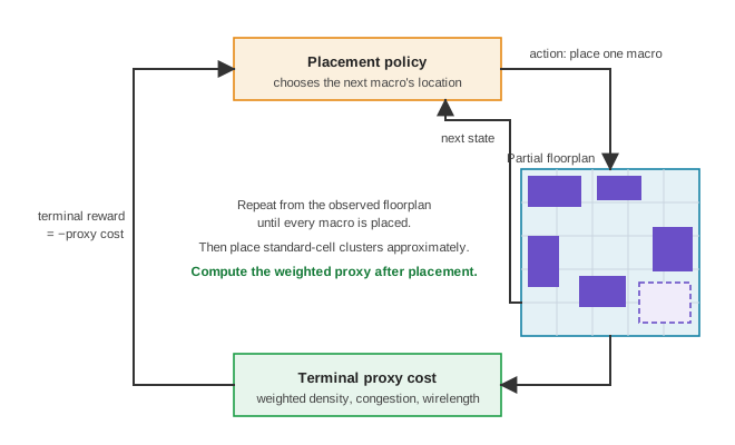
Reinforcement learning is plausible here because each macro placement alters the state that conditions subsequent actions (Figure 5.8). The policy emits one macro-location action at a time and receives the updated partial floorplan back as the next state; once all macros are placed, an approximate standard-cell placement produces a weighted proxy cost over cell density, wirelength, and routing congestion, and the negative of that cost is the terminal reward. Keeping action selection, partial-state return, and terminal evaluation distinct keeps us from mistaking proxy rewards for final signoff verification.
Search tactics can trade early sample efficiency against later improvement, but that trade does not belong to one method family in the abstract (Figure 5.9). The constructed profiles isolate four possible budget-response shapes without assigning them to language-model prompting, Bayesian optimization, reinforcement learning, or random search. An actual method earns one of these descriptions only through measurements on the declared design space, tuning effort, and evaluation path.
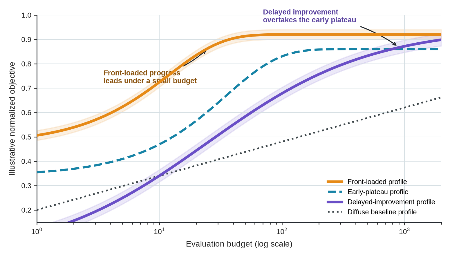
The four constructed profiles make one bounded point. A strategy can lead under a small evaluation budget and lose under a larger one, so early sample efficiency and later improvement must be measured separately (Figure 5.9). The curves do not tell us which algorithm will follow which profile. That depends on the design representation, tuning effort, randomness, evaluator, and stopping rule. Placement-stage proxies can guide the search, but they do not cover every downstream routing, timing, or manufacturing effect, so later checks must address those missing properties.
Because our architectural objectives constantly conflict, we evaluate tradeoffs by checking for dominance. One evaluated design dominates another when it proves no worse on every declared objective and strictly better on at least one. The Pareto frontier simply contains all of our evaluated designs that are not dominated by any other (Deb 2001). Using multiobjective optimization, we can expose the raw tradeoffs among power, performance, area, reliability, or cost, rather than hiding them behind a single, artificially weighted score. But the frontier itself never chooses the final design. As architects, we still have to decide which specific tradeoff fits our system constraints, whether our declared objectives actually capture what matters, and which unevaluated regions remain too uncertain to trust. Depending on what we learn, our most useful output might be a single candidate, a broad Pareto region, a mapped constraint boundary, a sensitivity analysis, a definitively ruled-out region, or simply the parameters for our next experiment.
Deb, Kalyanmoy. 2001. Multi-Objective Optimization Using Evolutionary Algorithms. John Wiley & Sons.
Our search procedures differ in the design-space structures and feedback costs they handle well (Table 5.7). For each procedure we pair its strong fit with the conditions it requires and the mismatch that disqualifies it, and that mismatch column is the practical rejection test: it keeps us from deploying a procedure whose mathematical assumptions contradict our physical design space.
| Search procedure | Strong fit | Required conditions | Common mismatch |
|---|---|---|---|
| Enumeration | Small, finite legal spaces where we can check every candidate. | Explicit action space and affordable complete coverage. | Trying to use it after our space has grown beyond our available budget. |
| Random search or sampling | Large spaces that permit independent samples and require a transparent control. | Legal sampler, matched budget, and retained failures. | Treating it as a guarantee against a poor objective or representation. |
| Deterministic heuristics | Spaces where we can exploit useful domain structure to reduce the search transparently. | Stated rules, assumptions, and clear stopping conditions. | Hiding our tuning, or using a rule whose bias blinds us to the most useful regions. |
| Bayesian optimization | Expensive black-box evaluations in low or moderate dimensions where we can maintain a useful surrogate and acquisition rule. | Compatible observations, a checked surrogate and acquisition rule, and a sequential budget. | Applying it to a highly combinatorial or shifting space where our surrogate fails. |
| Differentiable optimization | Continuous parameters or a trustworthy differentiable relaxation of a discrete problem. | Useful gradients and a plan to check the relaxed solution after we discretize or implement it. | Ignoring the proxy or relaxation gap, letting the gradient point us toward an unrealizable or inferior design. |
| Evolutionary search | Discrete or mixed spaces where we can leverage populations, mutation/crossover structure, and parallel evaluations. | Legal variation operators and a massive evaluation budget. | Starving the population of evaluations, using opaque tuning, or running weak comparisons against random/local search. |
| Reinforcement learning | Genuinely sequential state-action problems that feature repeated related tasks and delayed feedback. | A state representation that preserves enough information to predict the next state and reward, plus a meaningful reward, affordable interactions or transfer, and a stable simulator. | Treating a static one-shot parameter search as RL when we have no sequential advantage. |
| Mathematical programming, constraint solving, or program synthesis/search | Algebraic objectives, discrete choices, or precisely specified legality and construction rules. | Executable objectives, constraints, or program semantics. | Hoping it will optimize for a broad architectural desirability that we never actually represented in our formulation. |
A familiar method name cannot repair a space, objective, or feedback path that violates the assumptions of our chosen search procedure.
Every time we deploy a learned optimizer, we must benchmark it against a strong, simple comparison running under the same legal space, tool path, and evaluation budget. For a small finite set, enumeration provides our baseline. For larger spaces, random search often proves useful because it requires no learned surrogate and parallelizes easily (Bergstra and Bengio 2012). If we have good domain structure available, a deterministic heuristic might make an even stronger baseline. Random search can still optimize a poor proxy or a badly represented space, so we use it as a transparent control rather than a guarantee of correctness.
Bergstra, James, and Yoshua Bengio. 2012. “Random Search for Hyper-Parameter Optimization.” Journal of Machine Learning Research 13: 281–305.
Roy, Rajarshi, Jonathan Raiman, Neel Kant, et al. 2021. “PrefixRL: Optimization of Parallel Prefix Circuits Using Deep Reinforcement Learning.” Proceedings of the 58th ACM/IEEE Design Automation Conference (DAC), DAC ’21, 853–58. https://doi.org/10.1109/DAC18074.2021.9586094.
PrefixRL, a reinforcement-learning framework for circuit synthesis, illustrates a much tighter sequential formulation. It explicitly casts parallel-prefix circuits as a reinforcement-learning problem, pulling logic synthesis directly into its evaluation path (Roy et al. 2021). When we combine a declared circuit space with rigorous synthesis feedback, we make our method inspectable. Even so, our final result still relies entirely on the quality of our objective, our tool conditions, and our matched baseline.
Our optimizer should finally stop when its budget is spent, when our decision stabilizes, when required inputs become unavailable, when the feasible region turns out to be empty under our declared constraints, or when another evaluation is simply unlikely to change our decision enough to justify the cost. In our execution request, we should always ask the environment to retain the rationale for why it selected each evaluation, as well as how the advanced method compared against our simpler baseline. If our selected optimizer relies on a generator to build legal candidates or a predictor to avoid expensive evaluations, those distinct jobs should dictate how we compose our final search architecture, rather than following a fixed method order.
5.8 Heterogeneous and Hybrid Optimization Methods
Real-world architecture design problems rarely fit neatly into a single method family. Complex hardware-software co-design requires composing predictive surrogates, generative candidate constructors, and search optimizers into hybrid, multi-stage pipelines. We do not enforce a rigid, universal sequence of prediction, generation, and optimization. Instead, we anchor our hybrid compositions directly in the missing capabilities of our specific design problem, allowing physical tool feedback to govern the workflow. In neurosymbolic architectures, for instance, we orchestrate probabilistic neural generators alongside symbolic logical verifiers, AST checkers, and analytical rooflines. Every added component in a hybrid pipeline must earn its place by performing necessary work that simpler conventional tools cannot execute economically.
In our systems, a predictor might condition a generator before construction, screen artifacts after generation, or sit inside an optimizer as a surrogate. We can design an optimizer to control a generator, select among existing candidates, or use direct tool feedback without any predictor at all. Likewise, a generator might revise an artifact immediately after a compiler or simulator returns its results. We can omit any of these families entirely, and our feedback loops can always route the work back to whichever component owns the required change.
We should not automatically treat generation, prediction, and optimization as a rigid three-stage pipeline. We combine them only when our problem involves distinct jobs. As we established when connecting intent to executable specifications (Section 1.4.2), tools like AutoTVM and Ansor illustrate successful optimization compositions in tensor-program tuning, but they do not establish a mandatory three-stage workflow across our broader architecture research (T. Chen et al. 2018; Zheng et al. 2020). We make these distinct jobs explicit in our worked comparison in Table 5.10. For instance, KernelBench needs generation and a harness, but not a learned optimizer, and we might conduct a small enumerated study that needs none of the three.
We routinely surround these compositions with other engineering roles. For example, if a critique identifies a missing AXI ordering assumption, we might use a learned method, a script, or our own engineering intuition to return a repaired artifact. We rely on interface and implementation tools to check stated properties, while our test harnesses coordinate compatible RTL, compiler, workload, and tool states. Our analysis methods, or our own insights as architects, help us explain whether data movement, computation, or another underlying mechanism actually changed the system result. Although these roles produce distinct outputs, we do not view critique, repair, checking, explanation, or coordination as additional method families. We do not require a learned component to perform any of them. Giving each of these roles a concrete output and a named next check or handoff makes its interface explicit across system compositions (Table 5.8) and keeps our engineering workflow independent of whichever software agent or human architect executes it.
| Engineering role | Concrete output | Next check or handoff |
|---|---|---|
| Proposal | A named candidate, artifact, or experiment request with the changed elements identified. | Check legality and scope before invoking an expensive tool. |
| Screening | A scoped estimate or ranking with its predicted property, applicable conditions, and uncertainty. | Send selected candidates to the declared measurement path and retain predictions and observations for qualification. |
| Search | The next candidate or experiment, its selection basis, and the remaining budget. | Hand the request to the environment without changing the objective or legal design space. |
| Critique | A testable defect, missing assumption, or conflict tied to a named artifact or claim. | Return it to the role that owns the revision; critique neither changes the candidate nor replaces the requested check. |
| Repair | A revised artifact or request linked to its parent and the change made. | Treat it as a new candidate and rerun checks whose inputs or assumptions changed. |
| Checking | A result from a named check for a named property and condition, including incomplete or unknown outcomes. | Hand the return to Chapter 7 to determine whether it is valid, what property it establishes, and what conclusion it supports. |
| Explanation | A proposed mechanism and the observations or alternatives it must distinguish. | Request a targeted contrast or measurement; do not substitute the explanation for a property check. |
| Coordination | An ordered set of requests with dependencies, budgets, artifacts, and candidate identifiers. | Hand the requests to the environment, which constructs and executes the tool requests. |
We should let method fit, rather than the raw number of roles, define our component boundaries. One component may perform several roles when its inputs, outputs, allowed actions, costs, stopping conditions, and required checks remain explicit. We should split the work whenever those requirements differ, or whenever a shared component would judge the assumptions it created. Separate components add a handoff, but they do not establish independent judgment by themselves. An independence claim requires a sufficiently different execution, checking, or review path, alongside a clear account of the assumptions that remain shared. Our study records must state exactly which requirements, data, code, tools, and failure modes we share and which we separate. The recurring hybrid pipeline configurations each pair a composition shape ranging from a direct tool path to a full three-stage generation, prediction, and optimization pipeline with the job that justifies it and the condition that keeps it minimal (Table 5.9). Each earns its place only when every component performs distinct, necessary work and keeps a clear condition for removal.
| Composition | When it is justified | What keeps it minimal |
|---|---|---|
| Conventional technique or direct tools | Existing calculations, builders, solvers, heuristics, or evaluations can perform the job economically. | Add no learned component unless it removes distinct work without weakening the check. |
| Generation only | Useful artifacts are missing and direct checking is affordable. | Stop when enough useful candidates exist or review becomes limiting. |
| Prediction only | Existing candidates need cheap screening before costly evaluation. | Retain the predictor only while qualification and confirmation cost less than direct evaluation. |
| Optimization only | A declared objective can guide selection over a space too large to enumerate. | Compare with a strong simple baseline and stop when further selection cannot change the decision economically. |
| Generation plus prediction | Candidate construction is needed, but most proposals cannot afford direct evaluation. | The predictor screens only the consequence for which compatible support exists. |
| Generation plus optimization | Candidate construction is needed, and the evaluation budget requires selective search, but no supported surrogate is available. | The optimizer uses direct feedback and each generated candidate still passes the declared checks. |
| Prediction plus optimization | A surrogate makes selective search economical under expensive feedback. | Keep the surrogate, acquisition rule, and later confirmation separately inspectable. |
| Generation, prediction, and optimization | Missing artifacts, costly evaluation, and selective search all limit the same study. | Each component has a distinct input, output, action, cost, and stopping condition. |
Neither size nor order makes our composition stronger. The combination we choose must fit the specific limiting work our study faces.
5.9 Optimization Method Case Studies
The true test of any architectural methodology lies in how its formal selection rules hold up under concrete engineering demands. Abstract method taxonomies can sound convincing in isolation, but physical hardware constraints, simulation budgets, and verification requirements quickly expose whether a chosen approach accelerates design discovery. To examine how prediction, generation, and search operate under realistic constraints, we contrast two representative architectural challenges, comparing high-dimensional compiler phase ordering against multi-fidelity memory hierarchy sizing.
5.9.1 Compiler Tuning vs. Cache Evaluation
When we apply our limiting-work test to our two worked cases, it leads us to opposite method decisions. We find that compiler phase tuning and microarchitectural search readily justify multi-component compositions, whereas our Lighthouse cache study only requires direct tool use. To see the compiler side, consider tuning phase ordering across compiler optimization passes in LLVM, an open-source modular compiler framework, or schedule templates in AutoTVM (T. Chen et al. 2018). In LLVM, selecting and ordering passes within the PassBuilder pipeline, enabling loop unrolling, auto-vectorization, or polyhedral loop transformations creates a massive search space. Given a fixed operator and target, candidate schedules far exceed what we can measure directly. A learned cost model predicts likely performance, search algorithms allocate costly measurements, and compilation combined with target execution checks the selected schedules. Searching NPU tile mappings or tuning CPU branch predictor table allocations likewise requires selective search guided by surrogate models. For these complex tuning tasks, we justify multi-component compositions. However, when we encounter a new workload or target, we still need a conventional baseline (such as default LLVM -O3 compilation) and a matched budget before selecting learned components.
Chen, Tianqi, Lianmin Zheng, Eddie Q. Yan, et al. 2018. “Learning to Optimize Tensor Programs.” Advances in Neural Information Processing Systems 31: 3393–404. https://proceedings.neurips.cc/paper/2018/hash/8b5700012be65c9da25f49408d959ca0-Abstract.html.
Our Lighthouse cache study presents the exact opposite shape. The three cache-capacity settings we proposed already define the entire candidate set, and our budget safely covers a direct SRAM screen followed by matched cycle-level evaluations. If we introduced a generator, it would construct nothing new; if we added a predictor, it would demand observations we do not possess; and if we deployed an optimizer, we would needlessly search a simple three-point comparison. Set side by side across the same decision parameters, the two domains resolve oppositely (Table 5.10): missing capabilities and candidate-pool size, not method reputation, govern whether a complex hybrid pipeline or a minimal direct tool path is justified.
| Decision parameter | Compiler-tuning candidate | Lighthouse cache study |
|---|---|---|
| Job | Construct or select a schedule that improves a declared operator on a named target. | Compare our specified 2 MiB baseline setting against our proposed 3 MiB and 4 MiB settings without widening the scope of the study. |
| Inputs and support | Requires a fixed operator or workload, a target hardware definition, a legal schedule or program space, compiler state, observations drawn from matching conditions, and an evaluation budget. | Three proposed l2.capacity settings, declared hardware, software, and workload identities, specific SRAM limits, and no retained observations from prior matching conditions. |
| Approach status | A plausible composition might use AutoTVM-style schedule templates, a learned cost model, and simulated-annealing search, or perhaps Ansor-style program construction, learned cost prediction, and evolutionary search. Our choice remains open until we fix our comparator and budget. | We use direct evaluation as our next action once our proposed configurations and tool path become executable. We request our declared SRAM screen followed by matched cycle-level evaluations for eligible settings. We add no generator, predictor, or optimizer. |
| Output and legal actions | Return an accepted schedule alongside its measured target result. We may change only parameters in the declared schedule or program space. | A future run returns modeled SRAM properties alongside matched cycle-level results. We may only select l2.capacity values of 2MiB, 3MiB, or 4MiB and we may not change any other architecture or software configuration. |
| Evaluator and later checks | Our compiler and target measurements evaluate the selected schedules under common semantics and conditions. | Our planned SRAM-model screen checks the declared physical limits. Our planned cycle-level simulation, cache modeling, and power modeling return the matched system results we need for our later comparison. |
| Feedback cost | We must account for cost-model fitting, candidate construction, search, compilation, target runs, and tuning review under a matched budget we have not yet declared. | Our declared budget allows three SRAM evaluations and at most four cycle-level executions, which includes infrastructure reruns, configuration checks, and review. We have not yet incurred any execution cost. |
| Fallback and stop | We must establish a credible conventional comparator, matched budget, fallback, and stopping rule before we decide if this composition is justified. We have selected none here. | If our configurations and tool path become executable, we compare all capacities directly, bypassing the SRAM screen if necessary. We stop when we resolve the decision, exhaust our eligible set, spend our cycle-level budget, lack a required input, or find no alternative that passes the SRAM limits. |
These parameters resolve our approach choice for the Lighthouse cache study, but they do not dictate our final architecture result. Our compiler tuning remains conditional because we must select the strongest practical conventional alternative for our actual operator and target, rather than merely inferring one from a generic method label. Before we begin learned tuning, we should lock in a compiler default, an optimized library, an expert schedule, or a conventional autotuner as our baseline. We apply the same rule to our prospective KernelBench comparison, where the strongest practical conventional constructor remains unresolved.
5.9.2 Lighthouse Evaluation Plan
Our evaluation environment must receive far more than a selected method. We keep its allowed changes, required tool roles, cost envelope, validation checks, and fallbacks tightly coupled to our approach (Table 5.11). The Lighthouse cache study concerns an L2 SRAM cache configuration for a 3 W mobile XR SoC with a RISC-V RV64GCV application cluster, a proposed TSMC N7 or N3 process target, die-to-die UCIe chiplet interconnects, and CXL memory-expansion interfaces. Explicit bounds on the allowed changes and tool contracts keep the direct evaluation plan inspectable and support later replay.
| Handoff detail | Lighthouse cache method decision |
|---|---|
| Selected approach | We use direct evaluation with no added method. We add no generator, predictor, or optimizer because our three proposed capacities already define our complete candidate set. |
| Allowed change | We change only l2.capacity among 2MiB, 3MiB, and 4MiB; we keep our declared hardware, software, workload, cache policy, memory system, and exclusions strictly fixed. Any other architecture or software change reopens our study. |
| Required tool roles | An SRAM model operating under our declared TSMC N7 or 3 nm-class process, voltage, and temperature conditions screens macro area and access time, while supplying our cache energy and leakage estimates. A cycle-accurate simulator (such as gem5) with cache and power models measures matched frame-time, cache misses, and subsystem-power consequences. |
| Cost envelope | We allow three SRAM evaluations and at most four cycle-level executions, including any infrastructure reruns, alongside our declared configuration checks and review. |
| Necessary checks and fallback | We must confirm candidate and condition identity. We reject capacities that exceed 3 W in modeled subsystem power, 1.5 mm2 in macro area, or 2.5 ns in modeled access time for the 3 W Mobile XR SoC. At most one candidate may advance, and it can only do so if it passes its physical checks (including static timing analysis in OpenSTA and power intent checks in UPF) and yields a qualified interval relative to the 2 MiB rerun baseline above zero. Thermal and IR-drop reviews remain independent later requirements. If our SRAM screen becomes unavailable, our fallback is a matched direct comparison of all three capacities within that same cycle-level budget. Chapter 7 governs our interval qualification. |
While our SRAM screen may protect scarce cycle-level evaluations, it cannot interpret the eventual system-level results. We should revisit our choice to skip an added method only if our legal cache space expands, direct evaluation becomes our limiting cost, and observations from matching conditions finally become available. In making this choice, our study merely rejects an unnecessary method; it does not reject AI-native co-design as a whole.
5.10 Common Pitfalls
Whether we select direct evaluation or deploy complex prediction, generation, and optimization pipelines, hardware design introduces subtle methodological traps that rarely arise in pure software optimization. The pitfalls below are failure modes we anticipate from the mechanisms developed in this chapter, not findings from a measured survey of practice. They stem less from algorithmic flaws in our neural models or search heuristics than from optimization mechanics operating on uncalibrated proxy metrics, disconnected from physical constraints and downstream verification checks. When surrogate models operate without property-appropriate safeguards, optimizers can exploit surrogate inaccuracies rather than discovering genuine hardware improvements.
- Proxy gaming in surrogate-driven design search: When we optimize architecture candidates against fast learned cost models or analytical throughput approximations, our search algorithms can quickly exploit regions where the surrogate is over-optimistic. The resulting candidates achieve strong predicted scores while failing timing closure or memory bandwidth checks during full simulation.6
6 The Optimizer’s Curse in proxy search: In decision analysis, selecting the maximum score among noisy estimates systematically selects for optimistic prediction error (Smith and Winkler 2006). Even if a surrogate model is unbiased on average across a broad design space, candidate ranking preferentially selects for extreme positive errors, causing realized hardware performance to fall short of predicted scores unless validated by an independent, high-fidelity check or bounded by conformal prediction intervals (Lei et al. 2018; Angelopoulos and Bates 2021).
Smith, James E., and Robert L. Winkler. 2006. “The Optimizer’s Curse: Skepticism and Postdecision Surprise in Decision Analysis.” Management Science 52 (3): 311–22. https://doi.org/10.1287/mnsc.1050.0451.
Lei, Jing, Max G’Sell, Alessandro Rinaldo, Ryan J. Tibshirani, and Larry Wasserman. 2018. “Distribution-Free Predictive Inference for Regression.” Journal of the American Statistical Association 113 (523): 1094–111. https://doi.org/10.1080/01621459.2017.1307116.
Angelopoulos, Anastasios N., and Stephen Bates. 2021. A Gentle Introduction to Conformal Prediction and Distribution-Free Uncertainty Quantification. arXiv preprint arXiv:2107.07511. https://arxiv.org/abs/2107.07511.
Unconstrained High-Level Synthesis pragma optimization: When we deploy automated design space exploration over High-Level Synthesis (HLS) C/C++ pragma spaces without physical bounds, we invite resource over-allocation. Methods that insert loop unrolling, array partitioning, and pipeline initiation interval directives can generate invalid code structures that crash downstream logic synthesis or exceed our FPGA block RAM capacities.
Kernel distance mismatch in discrete microarchitectural Bayesian optimization: When we apply standard Bayesian Optimization (BO) with continuous Gaussian Process kernels to discrete hardware parameters, we risk severe kernel collapse. When our BO evaluates high-dimensional architectural choices like cache associativity, queue depths, and bus widths, continuous distance metrics can misrepresent parameter dependencies and stall our search efficiency.
Policy collapse and sparse reward failures in RL-driven microarchitecture search: When we train Reinforcement Learning (RL) agents on multi-stage hardware layout or instruction scheduling tasks, we struggle with long action horizons and sparse reward feedback. Without dense intermediate physical metrics, our RL policies can collapse into invalid action loops or fixate on narrow, non-generalizable design corners.
Un-synthesizable RTL generation in LLM code synthesis: When we rely on Large Language Model (LLM) generators trained on generic code bases, they can output hardware descriptions that appear syntactically correct but violate hardware legality, a failure class documented directly by the RTL generation benchmarks introduced earlier (Liu, Pinckney, et al. 2023; Lu et al. 2024). Such generators hallucinate non-existent IP interfaces, introduce unhandled race conditions in multi-clock domains, or produce Verilog constructs that fail our formal equivalence checking.
Liu, Mingjie, Nathaniel Pinckney, Brucek Khailany, and Haoxing Ren. 2023. “VerilogEval: Evaluating Large Language Models for Verilog Code Generation.” IEEE/ACM International Conference on Computer-Aided Design (ICCAD). https://arxiv.org/abs/2309.07544.
Lu, Yao, Shang Liu, Qijun Zhang, and Zhiyao Xie. 2024. “RTLLM: An Open-Source Benchmark for Design RTL Generation with Large Language Model.” Proceedings of the 29th Asia and South Pacific Design Automation Conference (ASP-DAC). https://arxiv.org/abs/2308.05345.
5.11 Open Questions
Transitioning AI-native co-design from an ad-hoc experiment into a rigorous engineering discipline requires resolving fundamental open research questions. While we understand the individual mechanics of prediction, generation, and optimization, we lack formal frameworks for prospectively quantifying method overhead, auditing surrogate validity, and triggering automated fallbacks when models drift. Addressing these research frontiers will determine whether learned components can achieve the predictability, accountability, and reliability demanded by production hardware workflows. Making learned components as accountable and predictable as the conventional evaluation paths they augment depends on crossing these barriers.
Prospective cost modeling and decision selection. To conduct a fair study, we need measurable ways to choose our approach before we know the actual results. This proactive selection ensures that our chosen method genuinely eliminates limiting work, rather than allowing prediction errors to masquerade as architectural gains.
Can we reliably predict when a learned method will actually save total design effort? To answer this, we need a prospective cost model that accounts for setup, data preparation, qualification, execution, checking, and expert review, using only the information we possess before the work begins. A successful solution would allow us to confidently choose a learned component over a conventional one, knowing definitively that it will reduce the realized cost of our study.
How can an architecture optimizer avoid being fooled by its own surrogate? Whenever we rank thousands of candidates, we increase the risk that the apparent winner simply happens to exploit an optimistic prediction error. Our open challenge is to design optimizers that reliably improve upon random search and survive independent, high-fidelity tool checks, all without expending the very evaluation budget we set out to save.
Auditing validity boundaries and world models. We can only rely on a learned method as long as its output respects our design constraints and operates within the bounds supported by our data and validation checks.
How can an architecture generator enforce hard constraints without destroying design diversity? We know that encoding rigid rules can filter out illegal structures, but doing so often unintentionally prunes away promising, unconventional alternatives. As architects, we still need methods that preserve a wide variety of legal candidates across different performance-cost regions, rather than maximizing the volume of valid outputs we can produce under a fixed evaluation budget.
When does an architecture problem actually justify building a world model? We know that building a transition model makes sense only if our actions change subsequent states and planning ahead saves us real evaluations. The open problem lies in defining exactly when the benefit of looking ahead across a growing action horizon outweighs the compounding prediction errors, setup costs, and checking overhead associated with static prediction or direct tool feedback.
Dynamic bottleneck adaptation and fallback triggers. Our composition strategies must change whenever an added method shifts the performance bottleneck instead of removing it entirely. Likewise, we should shrink our composition whenever a component no longer justifies its cost.
How can an automated flow adapt its own method composition as the bottleneck moves? Adding a generator might instantly shift our limiting work over to the simulator, while a fast predictor might just build up a queue for expert review. The open challenge here is to build systems that recognize these shifts and dynamically reconfigure their component mix to minimize total work. They must do this without abandoning our necessary cost accounting, fallback paths, and stopping conditions.
What signals should trigger an architecture flow to drop a learned component and fall back to a simpler tool? A learned component ceases to be useful when its support assumptions fail, when direct evaluation becomes cheaper, or when checking costs rise too high. The truly difficult part is distinguishing a fundamental structural shift in our limiting work from a temporary setback. We need mechanisms that trigger a fallback early enough to prevent wasted effort, while still retaining the components that actively improve our decisions.
5.12 Summary
In this chapter, we established that choosing an AI method for hardware design is an exercise in algorithmic parsimony. We must start with the specific bottleneck limiting our engineering progress, rather than selecting a model family based on industry trends or superficial appeal. Whether we deploy prediction to estimate expensive metrics, generation to construct missing candidate artifacts, or optimization to search vast design spaces, every added component must earn its place by removing concrete limiting work without creating unmanageable verification overhead.
Direct evaluation and conventional heuristics remain our default starting line whenever they can settle an architectural decision within our declared budget. When we do justify adding learned or hybrid components, we must ensure they preserve explicit downstream verification checks, clear fallbacks, and stopping conditions. When we evaluate this phase of Architecture 2.0, four core takeaways govern our work:
Key Takeaways: Matching the Method to the Limiting Work
- Minimal sufficient approach. Select the simplest method that addresses the active bottleneck, defaulting to direct evaluation or conventional tools whenever they fit the computing budget and verification needs.
- Limiting work drives method choice. Match prediction to costly evaluation, generation to candidate construction, and optimization to large legal search spaces, ensuring no added method enters the pipeline without a clear job.
- Surrogate qualification and support. Predictive models require qualification against reference tool observations within their specific design region, treating world models as transition-aware surrogates rather than universal architectural theories.
- Integrity through external checks. Every generated or optimized candidate must face a named, property-specific check whose assumptions, scope, and independence are explicit, backed by fallbacks and stopping rules when surrogates drift.
With our selected approach in hand, we now need a tool-connected environment capable of preserving allowed changes, enforcing required tool roles, maintaining cost envelopes, and executing necessary checks. We develop precisely that environment in Chapter 6.