4 Architecture Data, Knowledge, and Representation

“The limits of my language mean the limits of my world.”
— Ludwig Wittgenstein, Tractatus Logico-Philosophicus (1922) (Wittgenstein 1922)
Author’s Note. Ludwig Wittgenstein tied the boundaries of language to the limits of our world. Our claim for architecture is more pragmatic; a method can only act on the design state we expose to it. If our chosen representation cannot express a coherence assumption, a software dependency, or a physical limit, no tool or technique can deliberately preserve it.
North-Star question
Unlike an image-classification dataset, which packages each item as an array of pixels alongside a label, we cannot reduce an architecture result to just a number and a name. When we look at a cycle count, timing report, or power estimate, we are looking at a measurement tied to a specific design, software image, workload, tool path, version, and set of operating conditions. Even if a design’s text closely resembles known valid examples, a single incorrect connection or flawed protocol assumption can invalidate it.
We wrangle architecture data across disparate formats: specifications, source code and Register-Transfer-Level (RTL) designs, traces, and the measurements our simulators, formal tools, synthesis flows, physical-design tools, prototypes, and silicon return. Review comments and rejected design alternatives preserve human decisions that never appear in a tool report. We must balance these sources, knowing they vary widely in their access latency, freshness, acquisition cost, coverage, and ground-truth authority.
When we talk about a representation, we mean the specific form that exposes selected properties of a source or design to a given method. We might represent part of an architecture problem using a native RTL file, a typed graph, a table of measurements, a retrieval index, or a learned embedding. Because no single format preserves everything, our choice dictates which relationships remain visible, which designs we can express, and which mistakes a downstream method might fail to notice.
As architects, we typically use representation to denote a semantic design abstraction or structural level, along with its legal objects and permitted transformations. Meanwhile, machine learning practitioners frequently use the same word to describe an encoding or learned feature space optimized for a specific task (Bengio et al. 2013). For us, the unifying test across both disciplines is identifying which semantics and distinctions survive long enough to inform our intended operations and verification checks. Building an AI-native computing system means we often need both exact design semantics to drive our traditional tools, and rich feature spaces to guide our learned methods. Consequently, our RTL, Intermediate Representations (IRs), constraint sets, graphs, and embeddings all preserve different properties. They serve distinct purposes, and we cannot blindly swap one for another.
Our raw sources only transform into useful data after we identify them, align their versions and units, record their extraction conditions, and verify that their labels or tool returns mean what our dataset claims. From there, some of that refined data crystallizes into durable project knowledge, while other elements remain live project state that must evolve alongside our checked-in designs, software, workloads, constraints, and unresolved issues. While an architecture foundation model can supply broad prior knowledge about general mechanisms and common design patterns, its weights do not, and cannot, contain the authoritative truth about our current project.
If we ignore these distinctions, we risk deploying methods that retrieve stale guidance, compare mismatched tool returns, or optimize encodings that drop controlling relationships. As the first technical building block of Architecture 2.0, machine-usable hardware representations preserve these explicit links so that upstream candidate state connects cleanly to downstream search methods, tool execution, and verification feedback. We need to inspect these links before we choose a method, connect a tool, or interpret a final result.
Learning objectives
This chapter establishes the following learning objectives:
- Identify essential conditions that separate architecture data from generic machine learning examples.
- Map dynamic workload phase behavior, tool results, and acquisition costs to executable design states.
- Build datasets that explicitly handle tool failures, hard physical boundaries, and missing outcomes.
- Separate durable knowledge from live project state to trace facts to authoritative sources.
- Formulate code, graph, and trace embeddings alongside explicit design structures.
- Construct world-model state representations that support multi-step planning without drifting from physical reality.
4.1 Dataset Properties for Hardware Architecture
When we begin gathering data for a modern hardware architecture, we immediately discover that our artifacts refuse to fit into neat, uniform arrays. In traditional Architecture 1.0 workflows, we tracked design state through fragmented spreadsheets, un-indexed simulation logs, and isolated Verilog files, treating tool returns as ephemeral, one-off checks. Architecture 2.0 aims to replace this disconnected practice with a machine-usable representation graph that unifies live project state, multi-fidelity surrogate models, and formal design provenance.
Unlike image pixels or text tokens in standard machine learning benchmarks, an architectural measurement never exists in isolation. A single timing report or cycle count is bound to a specific RTL revision, compiler flag set, workload trace, tool version, and operating corner. If we attempt to treat a specification paragraph, a SystemVerilog module, a performance counter trace, and a routed timing report as interchangeable rows in a table, we strip away the physical and software context that gives those measurements meaning. Rather than dismissing these variations as noise to filter out, we must recognize that their differences define the data itself.
Our datasets also carry intertwined dependencies across their rows. We frequently see multiple results stemming from the identical design ancestor, generated artifact, workload trace, software image, tool model, or even an earlier architectural decision. For instance, if our physical-design run fails, we might get no complete metric at all; conversely, a timing check might only confirm whether we crossed a specific threshold. If we were to count these records as independent, neatly labeled examples, we would end up masking their underlying lineage and ignoring why certain values are missing.
When we evaluate architectural correctness, we face an unforgiving boundary. A model might generate a plausible token sequence that nevertheless connects the wrong signals, violates an interconnect protocol, drops a critical reset condition, or references a stale module hierarchy. Merely showing the system more superficially similar examples will not repair these broken relationships. To build a usable representation, we have to preserve the structure and contextual conditions that allow our tools, or our fellow reviewers, to spot such mistakes.
In our daily workflows, we often leave our sources scattered across separate project systems. We do not need to mash every configuration schema, workload manifest, repository revision, run directory, and review record into a single monolithic database. But we must establish shared identities, which allow another architect to look at our results and confidently determine which artifacts and measurements belong to the same design and operating conditions.
One transformation pipeline carries our architectural sources into method-ready representations without surrendering source authority (Figure 4.1). We convert raw heterogeneous sources (specifications, RTL, traces, EDA reports) into a checked dataset, distill verified facts into durable knowledge while keeping current parameters grounded as live project state, and finally expose those facts to downstream optimization or prediction methods through linked native, structured, or learned views. Source identity, versions, acquisition conditions, and access limits stay attached across the whole handoff, so we never treat derived encodings as interchangeable replacements for our authoritative sources.
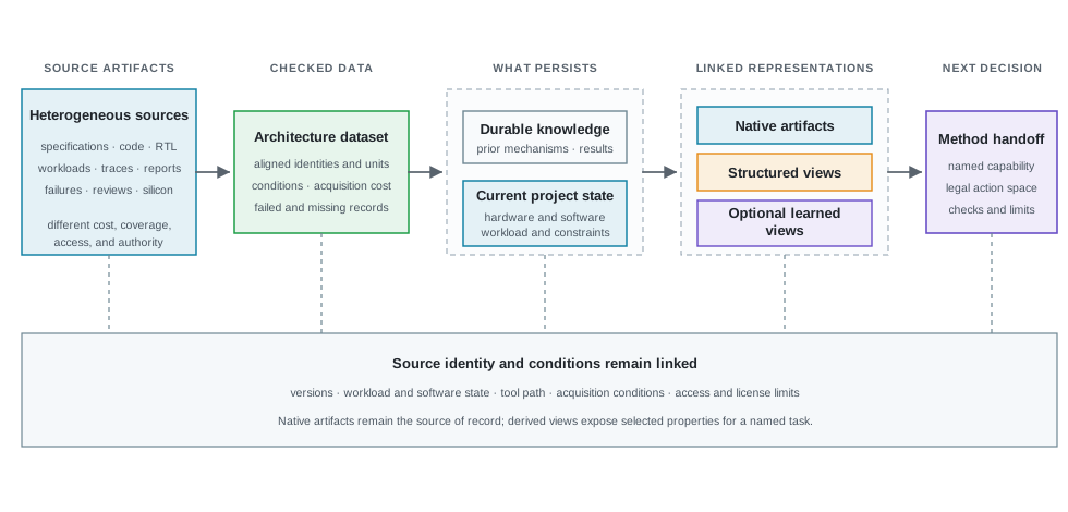
Our checked observations record exactly what a source returned under specific, documented conditions. Only our responsible project source gets to dictate which fact applies at any given moment. Because we can never assign either of these roles to an artifact with an unknown origin, our work must start by identifying our sources and clarifying what questions each one is equipped to answer.
4.2 Heterogeneous Architectural Data Sources
As we collect evidence across a complex design project, our data arrives from a wide array of media. Specifications articulate high-level requirements, source code and Register-Transfer-Level (RTL) netlists define executable hardware, instruction traces capture dynamic workload behavior, and electronic design automation (EDA) signoff reports record physical realities like area, timing slack, and power integrity. Beyond these automated outputs, engineering review notes and rejected design alternatives preserve human design rationale that never appears in a tool log. When we assemble these diverse sources, the challenge is not simply converting text and numbers into a common database format. Ten representative architectural data sources each pair a structural format with the properties it can preserve and the context it cannot establish in isolation (Table 4.1). For instance, while a paper or specification preserves high-level requirements and rationale, it cannot prove that a local netlist satisfies those requirements. Conversely, a gate-level netlist captures pin-level technology mapping and logic depth, but remains entirely blind to high-level design intent or dynamic software behavior. We must evaluate which specific architectural question each source is qualified to answer before connecting its observations to our active project state.
| Source structure | What it can preserve | What it cannot establish alone |
|---|---|---|
| Paper, manual, or specification | Concepts, requirements, interfaces, prior findings, and source-linked rationale. | The current project version or whether a local implementation satisfies the requirement. |
| Question and answer or design note | Focused reasoning, calculations, and review rationale. | Executable state, complete dependencies, or conditions not written into the note. |
| CPU or GPU compiler Abstract Syntax Tree (AST, in LLVM, Triton, CUDA) | High-level control flow, language AST nodes, thread-block tiling, and memory swizzling constructs. | Target microarchitectural execution timing, resource contention, or lower-level physical constraints. |
| Neural Processing Unit (NPU) Control-Data Flow Graph (CDFG) | Data dependencies, tensor operation pipelines, loop tilings, and scratchpad memory staging across NPU tiles. | Gate-level timing, physical layout congestion, dynamic power delivery, or unexpected host-side latency. |
| Code, RTL, or typed intermediate representation | Concrete structure, parameter values, interfaces, and buildable state within the properties the format expresses. | Workload coverage, design intent, or physical effects that require later tools. |
| SystemC and TLM 2.0 virtual platform model | High-throughput transaction-level memory and interconnect modeling, sockets, and early software bring-up. | Pin-accurate signal timing, clock-cycle physical delays, or lower-level gate/layout parasitics. |
| Gate-level netlist or technology-mapped cell graph | Technology mapping, pin-level structural interconnect, logic depth, and primitive cell allocations. | High-level architectural intent, unsimulated functional correctness, or post-layout interconnect parasitics. |
| Microarchitectural and memory trace (ChampSim, Ramulator) | Observed instruction execution, cache access patterns, and cycle-level DRAM bank/rank bus commands. | Behavior outside the captured trace population or system responses modified by timing feedback absent from the trace. |
| Tool run and report | A result under a particular design, tool, configuration, seed, model, and workload. | A general rule beyond those conditions. |
| Rejected candidate or review decision | A boundary that mattered, the conditions that exposed it, and the reason work stopped. | Whether the same rejection still applies after the design or conditions change. |
Because each source preserves certain relationships while leaving other claims unsupported, piling on more volume will not fix the gaps. We cannot make one type of data structure authoritative for domains it inherently does not cover. When we design a study for a general-purpose CPU core, an NPU tensor engine, or a High-Bandwidth Memory (HBM) controller, our source discovery should trace the exact architectural path that our decision crosses.
- Software and Compiler Stack: At the top level, application binaries and execution traces capture dynamic phase behavior. Frontend compiler ASTs (in Clang/LLVM, Triton, or CUDA PTX) expose control structures, thread-block tiling, and software transformations. Hardware-oriented compiler representations (such as NPU CDFGs in Spatial IR or MLIR dialects) capture tensor operation dependencies, systolic array loop-nest tilings, and scratchpad SRAM buffer allocations.
- Microarchitecture and Simulation Stack: Transaction-Level Modeling (TLM 2.0) virtual platforms supply transaction representations for early software bring-up without pin-level clocking. At the microarchitectural level, cycle-accurate full-system simulators (gem5), systolic-array accelerator simulators (SCALE-Sim), trace-driven simulators (ChampSim and Ramulator 2), and compiled HDL simulators (Verilator) expose core interface counters, bus contention, and queue dynamics.
- Physical Synthesis and Signoff Stack: Native RTL, technology-mapped gate-level netlists (synthesized cell graphs from Yosys or Design Compiler), SystemVerilog Assertions (SVA) paired with Bounded Model Checking (BMC) in formal flows, and coverage databases validate physical implementation. Physical synthesis and static timing analysis (STA) from OpenROAD and OpenSTA, alongside commercial power integrity tools, inject physical signoff results. Finally, emulation platforms, FPGA prototypes, and post-silicon tests validate deployed behavior.
We must treat expert judgment as just another form of conditioned data. If we want our judgments to be reusable, we have to record the evidence presented to the expert, the criteria they applied, their role and expertise, their confidence level, and any lingering disagreements or limiting context. When we make a schedule-driven compromise, fall back on a local convention, or rely on a rough estimate, we must label it as such, rather than letting it quietly harden into accepted architectural fact. We will explore whether those judgments can reliably support later claims in Chapter 7.
While all these sources map out the information that might exist in our environment, we face a separate set of constraints when it comes to securing access, obtaining permission to use that data, and ensuring that another group can independently verify our claims.
4.3 Data Licensing, Privacy, and Provenance
Even after we align the semantic properties of our data sources, we encounter a practical barrier. Hardware data is rarely freely shareable or unconstrained. The authoritative sources of truth in industrial architecture work are almost always governed by strict foundry Non-Disclosure Agreements (NDAs), Process Design Kits (PDKs, such as TSMC N7 or N3 3nm kits that package foundry-specific transistor parameters, design rules, and cell layout models), and proprietary Electronic Design Automation (EDA) intellectual property (IP) abstracts. We cannot simply swap out a confidential commercial 3nm cell library for a convenient open-source alternative and expect our learned models or surrogate tools to yield valid production guidance. Instead, our representations must explicitly retain the original source identity, PDK revision, foundry NDA scope, EDA tool license terms, responsible owner, access limits, and specific operating conditions, complete with an immutable provenance link that an authorized reviewer can inspect and verify.
Artifact-level license and permitted-use metadata distinguish mere filesystem access from legal authorization to use a source for AI model training, retrieval, transformation, redistribution, or derivative publication. We must preserve foundry NDA boundaries, PDK distribution restrictions, commercial IP licensing (such as PCIe/DDR controllers, standard cell macro timing libraries, and Liberty/LEF files), and tool vendor terms alongside any derived datasets, retrieval indexes, learned representations, and model weights (Longpre et al. 2024). A PDK or commercial IP block licensed for internal chip implementation cannot be fed into external commercial LLM endpoints or public pretraining corpora. When applicability remains uncertain under complex foundry NDAs or EDA license agreements, we should seek legal review rather than assuming that model training or transformation erases the underlying contractual restriction.
Generated-output provenance and project confidentiality raise boundaries of their own for EDA workflows. We must retain the retrieved passages, supplied design context, model endpoint identities, and similarity checks used to examine generated RTL, synthesis scripts, or timing constraints. These records expose our known inputs and flag potential verbatim reproduction of proprietary IP blocks or NDA-protected PDK collateral. Separately, even when an IP block or PDK is authorized for internal design execution, netlist fragments, SPICE models, Liberty .lib files, or P&R reports may be prohibited from leaving secure computing enclaves. Therefore, we require explicit access, egress, and retention rules for our model endpoints, retrieval indexes, logs, and local caches.
Outside-review access introduces another consideration when working under foundry NDAs. Even when we cannot release raw foundry PDKs or proprietary IP netlists, we can still design reproducibility directly into our public claims. We can publish data schemas, collection procedures, workload definitions, artifact hashes, aggregate statistics, tool version identities, executable harnesses, and held-out evaluation policies while keeping NDA-restricted collateral safely inside approved enclaves. When we provide a public subset based on open PDKs (such as SkyWater 130nm or IHP 130nm), we allow independent groups to test whether comparative results reproduce. Our releases must clearly state which claims can be verified using open material and which remain tied to private foundry NDA evidence.
Datasheets for Datasets provides a standard methodology to document why a dataset was created, what it contains, how it was collected, and how its access is governed (Gebru et al. 2021). For hardware architecture AI datasets, a dataset card must explicitly track foundry PDK revisions, NDA boundary scopes, cell library licensing, EDA tool execution terms, failed or censored runs, and exact verification claims. Documenting these foundry NDA and EDA IP constraints ensures another architect can evaluate what a dataset represents without violating proprietary licensing boundaries.
While documentation states what our collection claims to contain and how we assembled it, acquisition context goes deeper. It establishes which source population, filters, tools, and measurement conditions actually produced the underlying records.
Real-world and fleet observations require even further acquisition context. We must record the deployed hardware and software versions, workload population, sampling policy, measurement conditions, privacy or redaction rules, and collection cost alongside the observation. A result from deployed systems exclusively describes that specific version and population; it does not automatically become a training label or a definitive conclusion about our next design.
Public availability serves as only the first filter, and the later filters in the OpenRTLSet collection pipeline remove far more than the first (Figure 4.2). The pipeline opens with approximately 103,000 permissively licensed public C/C++ repositories. The authors’ synthesizability screen shrinks that population to roughly 12,000 repositories, and their Vitis HLS (a Xilinx high-level synthesis tool) flow yields valid Verilog from only about 1,000 (J. Wang et al. 2025). Those 1,000 surviving repositories produce roughly 24,000 extracted Verilog modules; because one repository can produce many modules, that count uses a distinct unit and acts as an annotation rather than a fourth attrition bar. Initial public code volume is deceptive: multi-stage synthesizability and EDA tool-flow attrition dictate the true yield of usable hardware data.
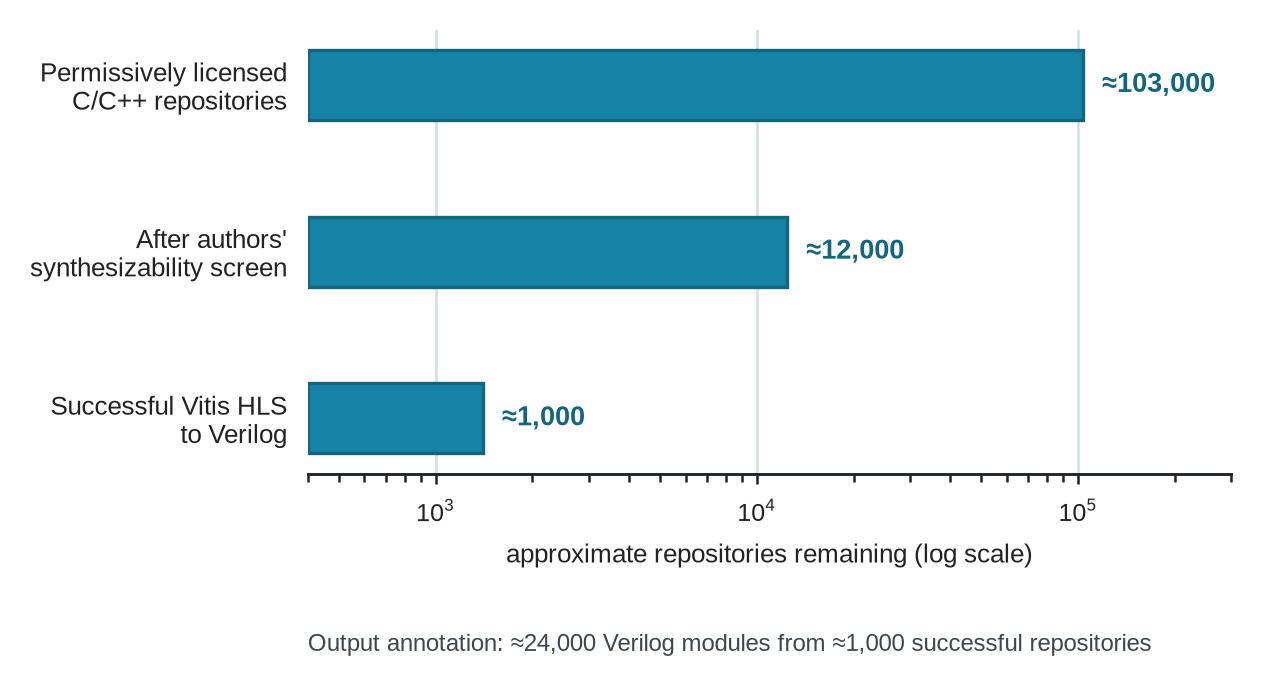
About 11.7 percent of the starting repositories survived the authors’ initial screen, and only about 1 percent successfully produced Verilog through this particular pipeline. Those derived ratios merely describe the authors’ specific repository search, license policy, screen, and tool flow, rather than estimating how much public C/C++ is synthesizable in general. The example makes a narrower point. Collecting public source code, deciding what is legally usable, screening it, executing a conversion tool, and accounting for failures are all distinct, necessary steps in our dataset construction.
Public corpus inventories use observation units that change with the task. General natural-language corpora report roughly \(1.5\times10^{13}\) tokens (Meta AI 2024; Together AI 2023), and open-source software corpora report roughly \(9\times10^{11}\) tokens (Lozhkov et al. 2024). Hardware collections instead count modules, layouts, or questions. OpenRTLSet contains roughly \(1.3\times10^5\) Verilog modules (J. Wang et al. 2025), CircuitNet reports on the order of \(10^4\) retained layouts (Chai et al. 2022), and QuArch contains architecture question-answer pairs numbering in the low thousands (Prakash et al. 2025). These quantities cannot be divided into a common scarcity ratio because a token, module, layout, and question are not commensurate observations.
The unit change is itself the architectural point. A large language corpus does not supply synthesizable modules, physical layouts, project histories, or checked architecture decisions. Reported hardware-generation failures, including nonexistent SystemVerilog syntax and invalid AXI interfaces, reinforce the need for domain curation and machine-checkable representations (Liu et al. 2024). They do not establish a numeric conversion between general text and architecture data.
To address these data volume disparities effectively, our representations must account for how different public datasets specialize across distinct abstraction tiers. Four representative public architecture datasets, OpenRTLSet, RTL-Repo, CircuitNet, and QuArch v0.1, each observe a different unit and support a different task, leaving different parts of our design decisions unobserved (Table 4.2). For example, while OpenRTLSet measures fine-grained Verilog module synthesis and CircuitNet observes back-end physical-design layouts, QuArch evaluates high-level architecture knowledge retrieval. Consequently, sample counts across these datasets are not comparable. Each dataset exposes a different facet of our design problem while leaving other hardware context unobserved.
| Collection and observation unit | Supported task | Key missing context | Failed or rejected data status |
|---|---|---|---|
| OpenRTLSet observes one extracted Verilog module from public Verilog, translated VHDL, or C/C++ passed through HLS (J. Wang et al. 2025). | Fine-tuning and evaluating module-level Verilog generation. | Full project state, workload and software conditions, physical measurements, per-module functional checks, and a repository-disjoint split are not established. | Failed VHDL and Vitis HLS conversions are excluded. The source does not report a released corpus of failed artifacts and structured rejection reasons. |
| RTL-Repo, a benchmark dataset for multi-file Verilog autocompletion, observes one target-line completion with the surrounding Verilog repository as context (Allam and Shalan 2024). | Long-context, multi-file Verilog autocompletion measured with exact match and edit similarity. | Functional, synthesis, simulation, workload, power, performance, area, and physical-design evidence. The reported train and test counts do not establish a repository-disjoint split. | No design tool is executed for the observation. Repositories rejected by the collection filters are not reported as retained records. |
| CircuitNet, an open-source dataset for physical-design prediction, observes one back-end design run and retained layout under a declared synthesis and physical-design setting (Chai et al. 2022). | Cross-stage congestion, design rule check violation, and IR-drop prediction from graph and image-like features. | Front-end software and workload behavior, live project history, and a canonical grouping rule for evaluation. | The authors attempted 12,960 runs and retained 10,242 layouts after excluding failed runs. Failure artifacts and causes are not reported as retained. |
| QuArch v0.1, a multiple-choice computer architecture benchmark, observes one expert-validated multiple-choice question-answer pair about a computer architecture topic (Prakash et al. 2025). | Evaluating architecture knowledge retrieval and fine-tuning language models for that task. | Executable design state, workload and software identity, tool returns, physical measurements, and signoff evidence. | Validation removes questions without definitive answers or with scope too narrow for the benchmark. Rejected questions and reasons are not reported as retained. |
Missing context is not the same as poor data quality. For example, QuArch can serve as a well-validated test of architecture knowledge without ever describing a live design project. CircuitNet, in turn, can provide executed physical-design observations without recording the behavior of the software that might eventually run on the chip. As architects, we must match our collection to the specific property and transfer claim, rather than treating public availability or a large sample count as sufficient evidence.
While public sources make broad comparison and reuse possible, they usually omit proprietary design context. Community datasets can preserve declared repositories, flows, and collection choices, yet their quality depends on what contributors choose to record and release. Our internal sources may carry the current design, review history, and vendor material that a real decision needs, but privacy, intellectual-property, license, and access limits constrain how we use them. Our datasets must preserve that access status rather than silently replacing a restricted source with a convenient public one.
ChipNeMo, an LLM domain-adaptation framework for chip design, provides us with a clear task-specific example. It adapted language models and a retrieval model using proprietary chip-design material, and then evaluated an engineering assistant, EDA script generation, and bug summarization inside that restricted setting (Liu et al. 2023). This example shows how our internal data can improve selected internal tasks. However, it does not establish a broad architecture-design capability, and its proprietary evaluation cannot substitute for an independently testable claim.
Through all of this, one source remains central to almost every architecture result we produce. The workload ultimately determines which parts of our hardware and software become active.
4.4 Workload Behavior, Trace Costs, and Execution Coverage
Static hardware netlists and microarchitectural specifications describe what a system can execute, but they reveal nothing about real-world performance until software runs upon them. The dynamic behavior of application workloads, ranging from initialization bursts and memory-bound phase shifts to compute-intensive loops, dictates which hardware paths become active and which resource bottlenecks emerge. To evaluate an architectural hypothesis or train an AI surrogate model, our data representations must capture far more than isolated cycle counts. We must explicitly bundle dynamic workload phase encodings, execution scale, sampling policies, and tool observation costs into a unified representation of execution state.
4.4.1 Workload Phase Encodings and Dynamic AI State
When an AI agent navigates an architectural search space or a surrogate model predicts performance, it cannot evaluate a hardware design vector \(x \in \mathcal{X}\) in a vacuum. System performance, power dissipation, and thermal behavior are joint outcomes \(y = f(x, w)\) of the hardware configuration \(x\) and the dynamic workload feature vector \(w \in \mathcal{W}\). If we alter the underlying application software or workload phase, the exact same hardware candidate can shift from being compute-bound to memory-bound.
To expose dynamic workload behavior to machine learning models without incurring prohibitive full-trace simulation overhead, we transform raw execution traces into compact feature representations. Phase analysis tools such as SimPoint extract Basic Block Vectors (BBVs), representing execution interval frequency distributions \(w_{\text{BBV}} \in \mathbb{R}^d\), and cluster recurring execution intervals into representative phases (Sherwood et al. 2002). Similarly, statistical sampling frameworks like SMARTS compute statistical confidence bounds over sampled execution slices (Wunderlich et al. 2003).
In an AI-native co-design workflow, these basic block vectors, memory stride histograms, and phase embeddings serve two distinct representation roles.
- Surrogate model conditioning vectors: They supply the dynamic workload context \(w\) to learned performance predictors, allowing a single surrogate model to generalize across diverse software applications.
- Dynamic environment state encodings: In agentic design loops, encodings of dynamic workload phases form the environment state \(s_{\text{env}}\) of the agent’s decision space, enabling the agent to reason about phase-dependent bottlenecks and workload context transfer.
For our prospective Lighthouse cache study, the workload state requires a versioned snapshot of our bursty extended reality (XR) application alongside its exact software image and frame boundaries. A static memory access trace captured under one software image cannot be silently substituted for another, because dynamic timing feedback between the microarchitecture and software interleaving alters the instruction stream. Our representation must explicitly bind the workload phase feature vector \(w_{\text{BBV}}\) to its software image, collection policy, stable frame identifiers, and underlying hardware execution parameters. Once we make these workload conditions explicit, we can evaluate what a single observation costs and which portion of our execution space it covers.
4.4.2 Observation Paths, Acquisition Costs, and Execution Limits
When we evaluate an architectural hypothesis, we can inspect our system through a wide spectrum of observation tools. Six representative observation sources sit in parallel rather than in a ranking, spanning analytical models, trace-driven simulators, cycle-level simulators, RTL and gate-level simulation, FPGA or emulation platforms, and fabricated silicon (Figure 4.3). Each source yields an observation with distinct coverage, acquisition costs, environmental conditions, and blind spots, and we cannot arrange them into a single linear hierarchy of fidelity. Post-layout static timing analysis captures sub-nanosecond gate delays that an FPGA prototype loses, yet an FPGA platform allows us to boot a full operating system and execute billions of workload cycles that gate-level simulation could never complete in a reasonable timeframe. Fabricated silicon provides direct observations of one implemented chip under named test conditions, but it cannot evaluate a counterfactual design variation that we chose not to tape out.
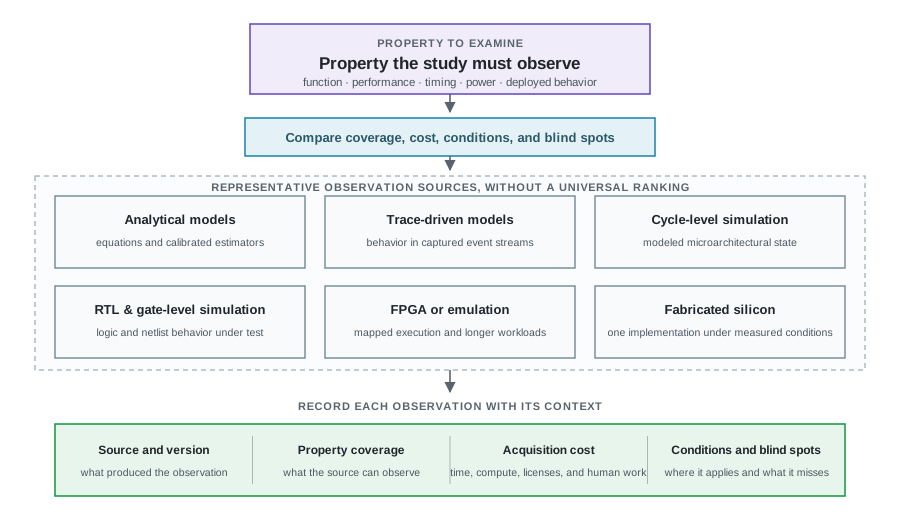
When designing our evaluation strategy, we start by defining the exact property we need to observe. We then evaluate candidate sources based on their coverage, cost, conditions, and inherent blind spots, often selecting a combination of several tools. We present these six sources in parallel rather than as a strict hierarchy because no single source is universally superior to the others. Every time one of these tools produces an observation, we must record the context required to interpret and compare that result accurately. Our choice of tool is dictated by the specific property and decision at hand, not by some generic ranking of fidelity.
Instead of exhaustively cataloging every possible return type, our overview groups the major observation paths we rely on in practice. Every observation source carries representation limits that must travel with its results, and Table 4.3 records them for the eleven we rely on. For example, while trace-driven simulators (like ChampSim or Ramulator 2) enable fast, repeatable studies of memory access streams, they cannot capture dynamic timing feedback absent from the original trace. We keep simulation, formal analysis, and implementation-facing flows separate because they yield different kinds of results.
| Source | Useful for | Important limit to represent |
|---|---|---|
| Analytical model | Fast sensitivity studies and early bounds. | Simplifying equations, calibration range, and omitted interactions. |
| SystemC / TLM 2.0 virtual platform | Rapid transaction-level memory and interconnect throughput exploration and early full-stack software bring-up. | Pin-level clock timing, detailed gate-level delays, physical layout parasitics, and unmodeled bus contention. |
| Trace-driven simulator (ChampSim, Ramulator 2) | Repeatable study of memory access streams, cache hierarchies, and DRAM bus scheduling under captured workloads. | No behavior that depends on timing feedback absent from the trace, and no unmodeled bus/interconnect states. |
| Cycle-level simulator (gem5, SCALE-Sim) | Detailed modeled microarchitectural behavior across CPU cores, NPU accelerators, and interconnects. | Simulator abstractions, unsupported states, calibration, and execution cost. |
| Technology-mapped gate-level netlist simulation | Pin-level logic verification, cell delay evaluation, and unknown-value (X-prop) propagation under synthesized netlists. | Testbench coverage, simulator runtime overhead, gate-level timing abstractions, and unmodeled layout parasitics. |
| RTL simulation (Verilator, VCS) | Logic, interface, and microarchitectural behavior over the exercised testbench and observed properties. | Stimulus and testbench identity, functional and code coverage, simulator version, and unmodeled physical delays. |
| Formal analysis (SVA / BMC) | Proof, counterexample, bounded-only, or inconclusive status for a stated property, model, and assumptions. | Exact property and assumptions, abstraction, proof method, bound or completeness argument, vacuity checks, and returned status. |
| Synthesis and static timing or power analysis (Yosys, Synopsys DC, OpenSTA) | Logic transformation, technology mapping, and timing, area, or power estimates within the executed flow. | Libraries, modes, corners, constraints, tool versions, physical approximations, and effects outside the analyzed stage. |
| Place-and-route and physical verification (OpenROAD, Innovus) | Placement, routing, extraction, timing, power-integrity, and physical-rule results for the implemented database. | Floorplan and routing state, extraction and signoff models, modes, corners, waivers, tool versions, and unmodeled manufacturing conditions. |
| FPGA or emulation platform | High-throughput functional or timing-model execution after mapping. | Mapping differences, compile cost, debug visibility, and non-transferable Application-Specific Integrated Circuit (ASIC) power or timing. |
| Fabricated silicon | Behavior of a physical implementation under measured conditions. | Limited design variants, observability, stepping, test conditions, and inability to answer counterfactual questions. |
We do not order these sources from best to worst. Instead, the specific property we are studying determines which trade-offs and limits we can accept, and whether we need to orchestrate multiple tools to get a complete picture.
As we gather data, acquisition costs dictate the shape of our resulting dataset. Expensive observation paths yield far fewer data points. We can only safely perform direct comparisons across observations that share compatible designs, workloads, tools, and environmental conditions. Dumping a large collection of incompatible reports into a repository does not create a dense, usable dataset for our current study.
A quick back-of-the-envelope calculation illustrates how rapidly coverage requirements multiply our acquisition costs. Using some illustrative assumptions, rather than attempting to model a universal simulator, let us assume a 1 GHz target, a 1 s measured interval, and 0.2 s of target-time warmup per run. We will further assume a cycle-level simulator rate of 100,000 target cycles per wall-clock second, three repetitions, four distinct workloads, and zero queue or setup overhead.
During a single measured interval, our target executes 1,000,000,000 cycles. At our assumed simulator rate, simulating those cycles alone demands roughly 2.8 hours. Serial execution cost \(T_{\text{serial}}\) combines target warmup cycles \(C_{\text{warmup}}\), target measurement cycles \(C_{\text{measure}}\), repetition count \(R\), workload count \(W\), and simulator execution throughput \(v_{\text{sim}}\) in target cycles per wall-clock second.
\[ T_{\text{serial}} = \frac{(C_{\text{warmup}} + C_{\text{measure}}) \times R \times W} {v_{\text{sim}}}. \tag{4.1}\]
Under the assumptions in Equation 4.1, our suite executes 14.4 billion target cycles and consumes 40 serial simulator hours. While target cycles and simulator rate dictate time per attempt, warmup requirements, repetitions, and workload coverage multiply the total expense.
To make this acquisition cost even more concrete, we can look at BOOM-Explorer, an automated design-space exploration framework for open-source RISC-V cores. For its dataset of 994 legal microarchitectures, each high-fidelity Very Large Scale Integration (VLSI) flow evaluation took approximately six hours at the low end, and well over fourteen hours at the high end (Bai et al. 2021).
Because of these varying expenses, we must store a detailed acquisition record alongside every result we generate. This record identifies the specific type and fidelity of the tool run, noting whether the execution completed successfully, failed, timed out, or required a retry. It also captures the exact seeds or configurations that produced our measurement. Whenever available, we should retain any uncertainty intervals reported by the source, as well as the execution time, queue time, compute overhead, memory footprint, and tool license consumption. We must also track the human effort required for setup, diagnosis, review, and repair. Ten analytical-model calls, ten cycle-level simulations, and ten physical-design runs might each generate ten rows in a table, but they represent vastly different investments of cost, coverage, and opportunities to observe system failures. Even when we lack an exact monetary cost, our representation should preserve these distinct resource metrics rather than collapsing them into a single opaque number or omitting them.
We keep these resource counts embedded directly within our representation because our subsequent work relies on them to choose appropriate methods, manage tool infrastructure, interpret measurements, and fairly compare complete systems. Whenever we store a result, we must document enough of its source conditions and acquisition cost so that any architect can confidently decide whether that result applies to their problem and understand exactly what it took to produce it.
A row in our architecture dataset must preserve far more than a simple value and a generic label. The common dataset simplifications all discard part of the true architecture sample, and every omission carries a concrete consequence for later use (Table 4.4). For instance, rather than assuming independent, interchangeable rows, an architecture sample explicitly preserves lineage to avoid counting dependent results as independent support. Every stored observation links its result to its specific design history, property checks, acquisition status, and consumed resources.
| Dataset simplification | Architecture sample | Consequence for later use |
|---|---|---|
| Cheap acquisition | Our results often require scarce licenses, long tool runs, fabrication, setup, diagnosis, and expert review. | We must record the resources and human work required to obtain, or fail to obtain, the result. |
| Fixed ground-truth label | Our simulators, verifiers, or physical tools return results for named properties at stated fidelities and under recorded conditions. | We must preserve the property, check, fidelity, and conditions for later interpretation. |
| Independent, interchangeable rows | Our results frequently share a design ancestor, generated artifact, workload trace, software image, model, seed, or earlier decision. | We must preserve lineage and avoid counting dependent results as independent support. |
| Missing data without structure | Failed, timed-out, and rejected runs are often selectively lost, while some violations reveal only that a threshold was crossed. | We must retain run status, failure reasons, and censored bounds rather than learning solely from successful survivors. |
| Matching attributes imply comparability | Two rows support a direct comparison only when we make their candidate identities and permitted differences explicit, and ensure the workload, software, tool path, and relevant conditions match. | We must treat results with uncontrolled differences as advisory context rather than drawing samples from the same comparison. |
These distinctions change what our stored dataset rows contain. For example, a timing row does not blindly attach a universal “correct” or “incorrect” label to a cache design. Instead, it preserves the exact status returned by a named timing check, bundled with the logic library, design constraints, operating corner, and tool state. When a result fails or goes missing, our dataset preserves the run status and failure reason rather than silently treating the design as poor. We must then review this context to determine whether the return indicates a hard feasibility boundary, a transient infrastructure failure, or an unusable measurement. The failed-run records we outline in Table 4.5 keep those possibilities separate. When we embrace these rich sample semantics, we establish clear rules for how we must construct and audit our datasets going forward.
4.5 Constructing Architecture Representation Datasets
Accumulating a large directory of simulation logs, Verilog files, and timing reports does not automatically create a usable architectural dataset. If we launch thousands of expensive tool runs without a clear sampling strategy, we risk spending our compute budget on redundant configurations while leaving decision boundaries unobserved. To build a dataset that supports architectural decision-making, we must structure our acquisition pipeline before executing our first simulator run. We must explicitly define the target architectural decision, identify the minimal required unit of observation, declare our workload coverage targets, and establish how we will capture and retain tool failures.
We keep these requirements tightly bound to our architecture decisions by following a compact dataset-construction sequence.
State the architecture decision and any transfer claim the dataset must support.
Identify the design, workload, software, and physical regions covered by that claim.
Choose sources that observe each required property under matching conditions.
Budget samples across source fidelity and acquisition cost.
Preserve source and candidate identity, lineage, failures, censoring, access, and licensing.
Split records by the coarsest shared ancestor relevant to the transfer claim.
Check raw returns, derived metrics, and representation limits separately.
Record the claims that the acquired data does not support.
The first four steps shape our acquisition strategy. The next three protect our identities, lineage, and evaluation splits, while the final step records the limits of our collection.
4.5.1 Multi-Fidelity Sampling
Long before we deploy an active learning algorithm or a learned surrogate model to explore an architectural design space, we must formulate a multi-fidelity sampling strategy. In hardware architecture, we rarely have the luxury of sampling our design space uniformly using high-fidelity tools. Instead, we must combine rapid, low-fidelity estimates from analytical equations with targeted, high-fidelity evaluations from RTL synthesis or cycle-accurate simulation. To ensure these mixed-fidelity observations blend safely, our acquisition plan must explicitly declare the legal design parameters, workloads, operating conditions, and coverage targets across all sampling tiers.
Active learning algorithms choose the next observation that provides the most utility given the data we have already collected (Settles 2009). In our domain, that observation usually means waiting for the costly result of a simulator, a formal tool, a synthesis flow, or a physical-design run, rather than just asking a human for a label. Multifidelity methods take on a different job. We use them to combine information from sources that vary in cost and accuracy, provided those sources estimate the exact same output or share an explicitly modeled relationship (Peherstorfer et al. 2018). For us, a cheap estimate and a costly tool result can only blend safely when they measure the exact same property under aligned design, workload, and operating conditions, or when we have explicitly stated and checked their relationship. We cannot treat unrelated outputs as multifidelity observations merely because they cost different amounts to acquire. While we can certainly use active learning and multifidelity methods together, combining fidelities does not inherently require us to adaptively select our next run.
We often see projects use the term synthetic data to describe four different objects that should never share the same status. First, a generated candidate artifact might be proposed RTL, a compiler schedule, a configuration, or a floorplan. We must push it through syntax, typing, interface, invariant, and tool-legality checks before we can evaluate its properties. Second, a simulated observation is a return from a named simulator for a specific candidate under recorded conditions, naturally inheriting that simulator’s abstractions and inherent biases. Third, a perturbed or augmented record represents a derivative of a real or simulated parent; we keep its lineage explicit so that related variants remain clearly dependent. Finally, when we substitute a predicted value for an unmeasured property, we call that an imputation. We always label imputations as predictions, complete with their model, training scope, and uncertainty, and never present them as observed or simulated values.
Complicating matters, teams also use the term to describe training records sampled directly from a learned generator. These records carry a fundamentally different status from the four objects above. Because no architecture tool actually measured a property, we cannot call it a simulator return. A Hardware Description Language (HDL) record remains proposed RTL until our executable checks qualify it. Unlike an augmentation, a learned sample might have no observed parent, and unlike an imputation, it produces a new record rather than simply filling a missing entry. Machine-learning experiments warn us that treating learned synthetic data as if it were real can impair downstream generalization (Van Breugel et al. 2023). In our architecture datasets, we therefore retain the generator, its training scope, our sampling procedure, and any checks we ran against real or tool-derived observations.
These objects fail us in distinctly different ways. A generator might overproduce familiar structures while missing rare but legal designs, whereas a simulator might hand us precise values derived from a biased or poorly calibrated model. Perturbations preserve many of their parents’ blind spots, and imputations often smooth over the very constraint boundaries that matter most. Because of these distinct failure modes, we must subject generated artifacts to legality checks, group our dependent variants by their ancestor, and calibrate any low-fidelity or predicted values against sources that offer stronger support for the targeted property.
CraftRTL, a synthetic data construction pipeline for Verilog, provides an example of how we can constructively use synthetic training data. It creates Verilog examples for non-textual specifications like Karnaugh maps, state transitions, and waveforms, while building targeted repair data directly from errors made by model checkpoints (Liu et al. 2024). The authors’ reported gains apply to the evaluated Verilog coding benchmarks. However, these gains do not automatically make a generated module functionally correct, connect it to a real workload, or guarantee synthesis, timing, power, or physical-design quality for our new projects. The construction method successfully enriches the training signal, but we still rely on executable checks to determine what a candidate actually supports.
We often rely on a common acquisition pattern. We apply cheap analytical checks to generated candidates across a broad legal region, and then we spend our costly observations right near constraint boundaries or decision crossovers. This cheap preliminary stage prioritizes our measurements without enlarging our supported claims. We constrain any claims to the specific design, workload, software, and physical regions where we calibrated the relationship, along with our explicit interpolation assumptions. Unobserved regions remain unsupported.
When we let a selector choose runs adaptively, the resulting dataset describes only the region that specific selection policy visited. Unless we provide a separate sampling argument, we cannot claim it represents the legal design space uniformly. We therefore recommend retaining the exact selection rule, its version, our available candidate set, and the observations we had on hand when we chose each run. The observations selected by the method serve as policy-conditioned evidence, updating our method under that declared policy. The reusable-holdout result offers us a strong precedent for protecting evaluation data when our analysis adapts to earlier answers (Dwork et al. 2015). In architecture, we add a critical structural requirement to that separation. Our protected boundary should always follow the transfer claim, targeting a specific design family, workload, software revision, or later time period, rather than just carving out randomly selected rows. If we want to make claims beyond our policy-conditioned observations, we must provide separately held-out groups or a clearly stated correction whose assumptions are justified for our chosen acquisition policy.
Throughout our acquisition process, we must retain every attempted point, failure, and censored return, while reserving design or workload groups that the selector cannot consume. These requirements let later reviewers distinguish broad support from dense sampling near a predicted optimum. While we cover method selection in Chapter 5, this chapter focuses on recording how those choices shaped our dataset.
4.5.2 Dataset Integrity and Construction Pipelines
Building a resilient dataset construction pipeline requires establishing unambiguous data identity before we record a single metric. In an active design project, performance numbers and timing slacks are constantly generated across distributed compute clusters and varying tool environments. If a single row in our dataset fails to record the precise hardware revision, software image, workload snapshot, tool version, and operating conditions that produced it, that measurement becomes useless, or worse, misleading. When we construct our ingestion pipelines, we must enforce strict schema checks, verify unit consistency, eliminate stale build artifacts, and validate lineage links to ensure that every recorded observation traces back to its exact parent configuration.
Machine-learning research into label errors treats a supplied label as a data quality problem, rather than hiding it inside model uncertainty (Northcutt et al. 2021). Work on data cascades further demonstrates how upstream data problems compound into delayed downstream failures (Sambasivan et al. 2021). For architecture data, our corresponding provenance chain runs all the way from the native artifact or tool return, through the parsed measurement and any derived label, right up to our final architecture interpretation. Each link introduces a distinct failure mode. Source corruption might damage or truncate our native return. Parser or unit errors alter its fundamental value. Stale or mismatched identities accidentally attach a perfectly valid return to the wrong design, software, workload, or tool conditions. An incorrect derivation can assign the wrong pass, fail, feasibility, or property label, even when our parsed value was correct. We define label quality to encompass the named design, workload, tool conditions, and property, rather than isolating just the final category. We ensure every computed attribute retains the raw return and the exact derivation that produced it, so another architect can always locate a broken link.
Our outcome categories must explicitly survive these checks. An invalid request, a dependency failure, an infrastructure failure, an incomplete run, a measured limit violation, a formal result, and an unknown outcome all answer fundamentally different questions. If we naively collapse them into a binary success label, we teach later methods that a broken license server and a physically infeasible candidate represent the exact same thing.
Public benchmarks inject yet another checking problem into our flow. Models trained on public HDL corpora have often already seen the standard benchmark solutions, a contamination pattern widely observed in common Verilog benchmarks (Z. Wang et al. 2025). We see identical concerns surface in broader language-model evaluation (Balloccu et al. 2024). Ultimately, a benchmark score cannot establish general design ability if the evaluated artifacts likely appeared in the training data. For us, held-out designs, source identities, and executable checks matter far more than sheer volume of examples.
We keep our held-out designs outside of study-specific training, tuning, and method selection until the final evaluation. While this separation reduces leakage from our current study, an opaque pretraining corpus means we can never prove a model avoided encountering a design. Randomly splitting rows also proves structurally weak whenever nearby rows share a repository, a generator, a workload trace, or a time period. To be useful, our split must expose the specific transfer we care about, whether that involves a new design family, a unique workload, or a later project revision (Kapoor and Narayanan 2023). We must always group at the coarsest relevant shared ancestor whose separation would leak information about our claimed transfer. For example, we keep a generator family intact rather than splitting its generated variants, and we preserve a trace capture in its entirety rather than arbitrarily splitting sampled intervals across training, tuning, and evaluation.
Our dataset construction pipelines ensure that every sample collection pipeline enforces these structural boundaries before data reaches our learned models.
At the end of this process, our finished dataset records provenance, versions, access and licensing conditions, acquisition costs, omitted populations, leakage risks, and the specific reason each missing value remains absent. While these checks cannot guarantee that the dataset will support every future use, they make our support boundaries and omissions visible. This allows another architect to independently decide whether our data applies to their problem. A checked dataset records exactly what our sources returned, not which project facts remain universally true today. For those current truths, we must look to the authoritative project sources that own them.
OpenRTLSet provides us with a cleanly executed example of this sequence. The authors first collected public Verilog, VHDL, and C/C++ repositories under licenses they deemed permissible for academic and commercial use. They screened the C/C++ sources to exclude constructs their flow considered unsuitable for synthesis, and then ran vhd2vl on the VHDL and Vitis HLS on the screened C/C++ sources while excluding any failed conversions. As shown in Figure 4.2, this multi-stage pipeline filtered the initial C/C++ repository population down to roughly 24,000 HLS-derived Verilog modules, one of three source branches whose union yields roughly 131,000 modules (J. Wang et al. 2025).
The authors then decomposed multi-module files, ensuring that a single Verilog module served as their primary dataset unit. Their released rows preserve the source repository URL and original license name, pair each module with a generated description, and directly support model fine-tuning followed by evaluation on VerilogEval, a Verilog code generation benchmark suite (J. Wang et al. 2025). Because the source does not report a repository-disjoint split or offer a released corpus of failed conversions, the resulting rows cannot certify functional correctness or preserve the full state of the source project. Consequently, this example supports a narrowly scoped claim by proving how we can transform a licensed public-code collection into a module-level Verilog training corpus via filtering, tool execution, cleaning, and labeling. However, it explicitly does not measure the general synthesizability of public code, nor does it represent the coverage we expect in industrial architecture projects.
CircuitNet brings our missing failures into sharp focus from another direction. The authors attempted 12,960 back-end runs but retained only 10,242 layouts after excluding the failed runs (Chai et al. 2022). While this reported exclusion does not conclusively prove that a learned model will suffer from bias, it elevates survivor-only coverage to a reasonable concern, an inference we draw from the retention policy rather than a measured result within the CircuitNet paper.
Our prospective Lighthouse cache comparison demonstrates how we specify this sequence prior to collection. We define our unit of observation as one 2, 3, or 4 MiB capacity candidate tightly bound to the declared design revision, software image, XR workload snapshot, simulator, power and SRAM models, and specific process assumptions. Our budget permits exactly one SRAM evaluation per capacity and four cycle-level executions (inclusive of infrastructure reruns), logging a distinct status for every single attempt. To defend a transfer claim, we would require a held-out design, a separate workload, or a later time period; without those distinct groups, our data supports only an isolated, within-study capacity comparison. Because we have retained no source packages or tool returns, our source access and licensing remain unresolved. This leaves our missing thermal, IR-drop, and workload-population evidence visible. The complete represented problem detailed in Table 4.10 ensures we retain our legal changes, our optional learned view, our accepted blind spots, and the precise method handoff.
4.5.3 Failed and Censored Runs
In standard machine learning datasets, missing values or failed records are often discarded as corrupted noise. Beyond validating clean data streams, however, our hardware dataset construction pipelines must handle missing or failed tool returns; throwing away failed tool runs introduces survivorship bias. If we retain only the timing-closed configurations while silently purging negative-slack reports, unroutable layout netlists, and rejected design alternatives, our learned models will perceive a design space where physical limits seemingly do not exist (Rubin 1976). A timing violation or a routing congestion error is not a bad data point; it is an observation that defines the boundary of physical feasibility. To build an accurate representation of a hardware design space, we must record failed, timed-out, and censored runs alongside our successful outcomes.1
1 Censored observation: The result establishes only that a value lies above or below a threshold rather than reporting the value itself (Klein and Moeschberger 2003). If our target-frequency test reports only a failure, we consider it left-censored because it establishes that the maximum sustainable frequency lies somewhere below our target.
A versioned execution history separates three tracking attributes (attempt status, candidate outcome, and project update) that a naive log would conflate (Figure 4.4). A tool invocation can complete successfully, advancing its candidate and committing a new project version; it can complete yet fail performance checks, leaving the candidate rejected without any project update; or it can complete on stale inputs, yielding no usable candidate outcome for the active comparison and making no project update at all. Keeping these attributes separate prevents our dataset cleaning routines from mistakenly turning a tool failure into design evidence or misinterpreting a completed measurement as a state change. We detail the specific lifecycle mechanics for advancing work and formally changing accepted project state over in Chapter 3.
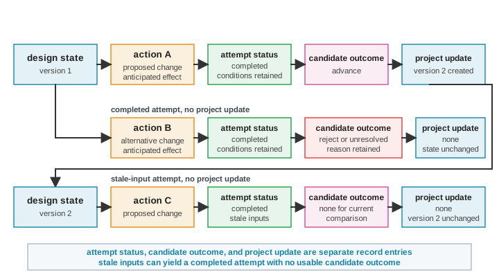
The branches depicted in Figure 4.4 illustrate our schema values rather than live Lighthouse outcomes. A prior result only transforms into a comparable sample when its design, candidate, workload, software, tool, and physical-condition identities fully satisfy our matching rules laid out in Table 4.10. Any other records can safely remain visible as advisory context without entering as samples for our current study.
We need negative records because our successful designs represent survivor samples. What we preserve from a failed run depends on how it failed, and Table 4.5 sets the preservation and consumption rules for seven failure categories. For example, when a synthesis or timing violation occurs, we preserve the candidate, constraints, process assumptions, and failing paths, ensuring we reconsider the candidate only after checking whether those exact conditions still apply. A robust record should preserve exactly why a run failed, without inflating a single localized result into a universal prohibition.
| Failed run or rejected alternative | What we keep | How our later work should use it |
|---|---|---|
| Synthesis or timing violation | Candidate, constraints, process assumptions, and failing paths. | We reconsider the candidate only after actively checking whether the relevant conditions still apply. |
| Unroutable or power-delivery failure | Netlist, placement conditions, density, congestion, or IR-drop result. | We identify the affected region and avoid treating the failure as a characteristic of all similar designs. |
| Proxy improvement overturned later | Cheap estimate, later observation, and the precise conditions under which they diverged. | We rigorously reassess the proxy’s useful scope before attempting reuse. |
| Tool failure or crash | Command, inputs, environment identity, logs, and failure classification. | We repair our environment without mistakenly recording the candidate as architecturally rejected. |
| Coverage gap | Missing workload, input, scenario, or architecture class. | We mark the strict boundary of the result rather than uncritically filling it with an assumption. |
| Reviewer rejection | Candidate, stated reason, risk, schedule, integration concern, and decision owner. | We preserve the rationale and revisit it only when the relevant conditions fundamentally change. |
| Waiver or exception | Violated rule, justification, scope, owner, and expiration or review condition. | We prevent repeated work while keeping the granted exception transparently visible. |
Our ability to reuse data later depends on the specific kind of failure we encounter. Timing, routing, or power-delivery failures might constrain a candidate when the exact same design and conditions recur. In contrast, a tool crash merely flags a need for environment repair and must never morph into a formal candidate rejection. Similarly, waivers retain their explicit scope, owner, and review condition, rather than quietly turning a temporary exception into a permanent, general pass.
4.6 Extracting Architectural Knowledge from Raw Data
Once we have constructed a clean, multi-fidelity dataset, we face an architectural distinction. Raw tool returns do not automatically constitute project knowledge or active state. In engineering practice, we often blur the boundaries between unparsed execution logs, verified design rationale, and the live configuration of our current chip revision. Yet, these three categories serve different roles in our decision loops. Raw data records what a specific tool returned under historical conditions; durable knowledge distills reusable design principles, verified specifications, and architectural rationale; and live project state defines the authoritative hardware, software, workload, and constraint parameters governing our work right now.
While our methods may need all three, these components change at different rates and originate from different responsible sources. For example, a paper can explain why cache capacity affects misses, but it cannot override our checked-in design. A retrieved manual can clarify a tool option, but it cannot establish which option our current run actually used. An old run can reveal a risk, but we cannot automatically substitute it for a current measurement.
An architecture foundation model brings broad prior knowledge learned across many sources. We can use it to retrieve a relevant mechanism, classify a familiar interface pattern, or identify which project document to inspect. However, it cannot supply the current design revision, software image, workload, constraint, open issue, or accepted tool result unless we feed those facts through a current, source-linked project context.
Because no single object owns every project fact, each preserves a unique kind of knowledge or state, carrying its own responsible source and freshness rule. The seven we rely on are collected in Table 4.6. For instance, trained-model weights supply general concepts as prior knowledge but cannot serve as the authoritative source of record for current project state. When we collapse these distinct objects into generic terms like memory or context, we obscure when one object should inform our decisions and when another remains authoritative.
| Object | What we preserve | Responsible source and our freshness rule |
|---|---|---|
| Trained-model weights | Learned statistical regularities and general concepts. | Useful as prior knowledge, but never the source of record for our current project state. |
| Retrieval index and retrieved material | Source-linked manuals, papers, examples, and project documents selected for our current task. | The underlying source remains responsible. Our version and date must match the use. |
| In-context working set | Instructions, selected sources, current state, and examples needed for one operation. | Transient assembly only. It does not become project state until a recorded update changes the responsible source. |
| Defined comparison | Question, comparator, scope, permitted changes, constraints, measurements, budget, and stopping conditions. | Remains our authoritative comparison definition until the owner records a revision. |
| Current design and software artifacts | Configuration, generated hardware, software image, manifests, and linked constraints. | Current only when our authoritative sources agree and consistency checks pass. |
| Workload state | Trace, profile, population, phase definitions, sampling policy, and version. | Controls the workload condition only within its recorded coverage. |
| Project history | Prior candidates, tool runs, failures, decisions, and rationale linked to their conditions. | Records what happened then, but does not make that result applicable to our current version. |
We cannot rely on a safe global rule that one file always wins. Our defined comparison states the permitted differences. The checked-in configuration and generated artifact define our implemented hardware state when they agree. The workload manifest identifies our current trace, while the specification states an interface requirement. A review decision records whether a candidate advanced. Because we draw each fact from its authoritative source, our projects cannot silently favor the most convenient one when those sources disagree. Instead, we must stop work until the owner reconciles the mismatch or records a revision.
We also see these objects change on different schedules. Model training captures general relationships over long periods, while retrieval supplies manuals and prior reports exactly when we need them. We must keep our current constraints in explicit project state, not embedded in model weights. Tool results only enter our project history after we know their identity and conditions. Fast-changing facts demand an explicit, versioned path. While slow-changing knowledge can inform our work, we cannot let it override those concrete facts.
Although our current working context assembles the subset of information needed for one operation, only a versioned change to an authoritative source can revise the comparison, design, workload, constraint, or accepted result. That change records its owner, dependencies, and consistency checks. We cannot turn advisory knowledge into current project state using fresh context alone.
Freshness itself draws the line between durable knowledge and live state. Split-brain causality names the failure where stale reference state \(V_1\) and current project state \(V_2\) generate an internally plausible yet invalid design proposal (Figure 4.5). A method reading stale reference specifications can propose a change that violates our active design parameters, and explicit version and freshness checks catch this mismatch before the proposal reaches a costly tool flow. Each file may look plausible in isolation, but together, unlinked freshness can describe a design that never existed.
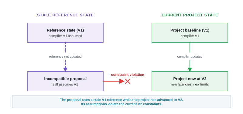
If we derive a proposal from reference V1, it can appear internally consistent while quietly violating the design we are developing at V2. We must catch that version mismatch to stop the proposal before it reaches an expensive tool path.
Our represented state can also drift from the artifact it claims to describe. If we rename a parameter in the generator, tighten a constraint directly in a Synopsys Design Constraints (SDC) file, or replace a block by hand, the state might still say it is current. Yet, regenerating the design produces something different from our checked-in artifact.
We can apply a direct check by regenerating the artifact from the represented state and compare our result with the repository. If the state cannot reproduce the design it names, we should not start work that depends on it. This check has a clear limit, though, because it only works where the state owns generation. If we make a hand edit below that level, we must detect it with another consistency check or make it an explicit part of our state.
To support these checks, our source identity needs enough detail. Depending on the artifact, we might require a version-control revision, content hash, tool and model version, workload manifest, seed, process corner, timestamp, or named owner. While our representation should keep only what our study needs, we cannot omit the identity required to decide whether two records describe the same conditions.
Keeping our current state accurate also carries a maintenance cost. A freshness check only reports a condition at one specific moment; it does not keep the state current. Every source that could change our decision needs a named owner and an invalidation trigger. Whether it is a new design revision, compiler release, workload capture, tool calibration, constraint, library, process assumption, or an expired waiver, any of these can make some part of our represented problem stale.
When an invalidation trigger occurs, the owner determines which dependent artifacts and results are affected. We might respond by regenerating an artifact, rerunning a consistency check, recapturing data, recalibrating a model, repeating a measurement, or marking the earlier result unavailable for our current comparison. These dependency links matter. They prevent a compiler update from forcing unrelated physical work, while ensuring that a changed cache generator correctly reaches all configurations, RTL, constraints, tests, and results that depend on it.
This maintenance consumes the same resources that our data acquisition does. Regeneration and checking use our compute, licenses, storage, and tool time. Recapturing a workload or recalibrating a model demands our data and engineering time. Broken links and source conflicts require us to diagnose and review. We should keep those recurring costs separate in the project record so we do not treat maintaining a rich representation as free, and so our later evaluations can see whether the retained state repaid its cost.
We should not maintain every source forever. When the refresh cost exceeds the value of keeping a source live, we can narrow the representation, freeze a versioned snapshot with an explicit review condition, or intentionally retain the missing relationship as a blind spot. A source without an owner, invalidation trigger, or affordable refresh path serves as historical context, not current project state.
Even with correctly separated data, knowledge, and live state, we cannot guide a method unless we expose the needed properties in a usable form. Our native artifact may remain authoritative while a derived encoding hides the very relationship that our task needs.
4.7 Hardware Representation Formats and World-Model State
Even when we have separated our raw data from live project state, we cannot pass an architectural design directly into a machine learning algorithm or optimization search without choosing a structural feature representation. The encodings we select, whether flat text tokens, Abstract Syntax Trees (ASTs), Control-Data Flow Graphs (CDFGs), physical layout matrices, or learned embedding vectors, dictate which design variations we can express, which structural dependencies survive, and which candidates our downstream methods consider similar. Raw text alone cannot safely capture complex hardware semantics, because small token edits in HDL source code can cause structural or physical failures.
We might describe an L2 cache resize, an NPU tile scheduling change, or a GPU kernel loop fusion in prose without ever identifying the specific configuration attributes, the affected interfaces, or the companion constraints. Tool-facing representations supply the structure we need. Parameter schemas enumerate legal values. Abstract syntax trees (ASTs) and Control-Data Flow Graphs (CDFGs) preserve critical structural and data-dependency relationships that a simple token sequence obscures. For CPU software and hardware-software co-design, Clang/LLVM ASTs expose control flow and language primitives before lowering into ISA instructions. For NPU acceleration, Control-Data Flow Graphs in MLIR dialects or Spatial IR capture tensor operation dependencies, loop-nest tilings, and scratchpad memory staging across accelerator tiles. For GPU kernel optimization, Triton and CUDA PTX compiler ASTs represent thread-block tiling, shared-memory layout swizzling, and Tensor Core scheduling. When we use typed intermediate representations, we can reject malformed constructions well before we pay the cost of expensive execution. Parameterized generators expose a bounded set of safe changes while retaining our lowering path to RTL.
However, typed representations are not universally safe. They only reject violations explicitly covered by their types and checks. When lowering across multi-level IR stacks (such as PyTorch/Triton \(\rightarrow\) MLIR Linalg/Vector \(\rightarrow\) CIRCT HW/HWModule \(\rightarrow\) SystemVerilog), each lowering step introduces lowering semantic entropy, where high-level structural semantics (tensor shapes, parallel loop iterations) are degraded into raw logic gates and wires, making reverse-engineering or post-hoc architectural verification difficult. For system-level multi-chiplet systems, specialized topology representations capture Compute Express Link (CXL 3.1), an open industry standard for high-speed cache-coherent interconnects, and Universal Chiplet Interconnect Express (UCIe), an open die-to-die interconnect standard, explicitly representing credit-based flow control, flit serialization latency, and NUMA memory hop penalties across chiplet boundaries.
SystemVerilog specifies logic, hierarchy, interfaces, and verification constructs (IEEE 2024). Technology-mapped gate-level netlists and And-Inverter Graphs (AIGs) generated by Yosys or Synopsys Design Compiler represent physical cell primitives, pin-level interconnect, and gate delays. Microarchitectural trace representations, such as ChampSim instruction traces and Ramulator 2 DRAM command logs, capture cycle-by-cycle memory access streams and bus contention. The Flexible Internal Representation for RTL (FIRRTL) and typed dialects within Circuit IR Compilers and Tools (CIRCT) expose operations, types, and compiler transformations (CIRCT Project n.d.; Izraelevitz et al. 2017). We also rely on companion formats like Synopsys Design Constraints (SDC) and the Unified Power Format (UPF) to carry our timing and power intent (Battu and Chugh 2024; IEEE 2025). Ten hardware representation formats each make specific design properties explicit while leaving others for downstream checks (Table 4.7). For instance, while typed hardware IRs (like FIRRTL or CIRCT dialects) explicitly enforce operations, types, and module connectivity, they cannot certify un-modeled physical realization or semantic intent.
| Representation | What it makes explicit | What still requires attention |
|---|---|---|
| CPU or GPU compiler AST (LLVM, Triton, CUDA) | Frontend control flow, language AST nodes, thread-block tiling, and memory swizzling constructs. | Target hardware execution timing, microarchitectural contention, and physical design feasibility. |
| NPU Control-Data Flow Graph (CDFG) | Tensor dataflow dependencies, loop-nest tilings, operator fusion, and scratchpad memory allocation. | Technology-mapped cell delays, clock-tree routing, power-grid integrity, and host interface overhead. |
| SystemVerilog or VHDL | Logic, hierarchy, interfaces, and behavior in the HDL. | Width conventions, connectivity, unknown values, verification intent, and all properties not established by compilation. |
| Technology-mapped gate-level netlist or AIG | Cell primitive assignments, pin-level connectivity, gate depth, and structural logic topology. | High-level architectural intent, unsimulated functional correctness, and post-layout interconnect parasitics. |
| Typed hardware IR such as FIRRTL or a CIRCT dialect | Operations, types, connectivity, and transformations supported by the IR. | Legal designs the IR cannot express, semantic correctness, lowering, verification, and physical realization. |
| Microarchitectural and memory trace (ChampSim, Ramulator) | Time-ordered instruction accesses, cache miss streams, and cycle-accurate DRAM bank/rank bus commands. | Behavior outside the captured trace population or system responses modified by timing feedback absent from the trace. |
| Parameter schema and generator | Named mutable parameters, legal values, and a reproducible path to generated artifacts. | Whether the generator and checked-in artifacts agree and whether dependent collateral changes with the design. |
| SDC, UPF, and other constraint collateral | Timing, power intent, domains, path references, and implementation assumptions. | Hierarchical-name coupling, stale paths, waived checks, and consistency with the RTL. |
| Graph or spatial representation | Connectivity, topology, adjacency, or physical location. | Properties omitted from nodes and edges, write-back to tool inputs, and physical rules not encoded in the graph. |
| Learned embedding or latent feature vector | Statistical similarity and directions learned from the data supplied during training or adaptation. | Exact artifact identity, hierarchy, topology, order, units, legality, constraints, uncertainty, source coverage, and check results. |
4.7.1 Code, Graph, and Workload Embeddings
When we deploy machine learning algorithms for retrieval, surrogate prediction, or design space search, we frequently project high-dimensional hardware artifacts into continuous latent feature spaces. We organize these learned vector representations across three core classes.
- RTL and code embeddings (\(\mathbf{z}_{\text{code}} \in \mathbb{R}^n\)): Token-level, AST-level, and retrieval embeddings (e.g. CodeBERT, ChipNeMo, RTL-Repo embeddings) that map SystemVerilog/VHDL source files into dense vector spaces for similarity search, code completion, and specification matching (Liu et al. 2023).
- Circuit and graph embeddings (\(\mathbf{z}_{\text{graph}} \in \mathbb{R}^m\)): Graph Neural Network (GNN) representations operating over And-Inverter Graphs (AIGs), technology-mapped cell connectivity graphs, MLIR spatial dialects, and physical floorplan adjacency matrices (e.g. DeepGate2 gate-level embeddings, learned macro-placement canvas graphs). These vectors encode structural topology, logic depth, and physical proximity (Shi et al. 2023; Mirhoseini et al. 2021).
- Workload and dynamic trace embeddings (\(\mathbf{z}_{\text{trace}} \in \mathbb{R}^k\)): Vector encodings of instruction streams, SimPoint basic block vectors (\(w_{\text{BBV}}\)), memory access stride distributions, and DRAM command logs.
While embeddings accelerate similarity queries and enable continuous optimization techniques (such as Bayesian optimization or gradient-guided search), we must treat an embedding as a derived auxiliary view, never a substitute for authoritative source code or native intermediate representations. Continuous latent spaces collapse exact syntactic rules, hard pin connectivity, and physical legal constraints. If an AI agent proposes a candidate design edit within a continuous embedding space, that update must round-trip back to explicit parameter schemas or native netlists and pass hard tool checks before entering our project record.
4.7.2 World-Model State Representations
Before an automated optimization method, search policy, or reinforcement learning agent can execute multi-step planning rollouts, our representation pipeline must define a formal state space. In Chapter 5, we introduce architecture world models, learned surrogate transition predictors that simulate environmental responses and structural consequences under proposed architectural actions. To enable these world models to conduct step-by-step design space rollouts without drifting into physically invalid states, this chapter establishes their foundational state space representation.
We define the complete world-model state vector \(s\) as a coupled tuple.
\[s = \left\langle s_{\text{design}}, s_{\text{env}} \right\rangle\]
- Design microarchitecture state (\(s_{\text{design}}\)). Represents the static structural hardware configuration. It combines explicit parameter tuples (such as
l2.capacity,noc.bus_width), typed intermediate representation graphs (CIRCT/MLIR dialects), cell-level And-Inverter Graph topologies, and learned structural graph embeddings \(\mathbf{z}_{\text{graph}}\). This vector explicitly carries the legal mutation boundaries and non-negotiable physical invariants of the design. - Environment and operating-condition state (\(s_{\text{env}}\)). Encodes the dynamic operational context. It incorporates workload phase feature vectors (\(w_{\text{BBV}}\) or trace embeddings \(\mathbf{z}_{\text{trace}}\)), process corner specifications (e.g. TSMC N3 SS/TT/FF corners), Unified Power Format (UPF) power domain states, Synopsys Design Constraints (SDC) clock maps, and thermal-power envelopes.
When an architectural agent executes an action \(a\), such as modifying an L2 cache capacity, adding a tensor tile to an NPU, or re-partitioning a clock domain, the world model evaluates the state transition \(s' = T(s, a)\).
To prevent multi-step planning rollouts from drifting into physically un-constructible regions, our state representation enforces three critical properties.
- State lineage and invariant preservation. Every intermediate state \(s'\) retains an immutable link back to its parent design revision, original PDK corner rules, and verification constraints, as formally structured in Table 4.10.
- Multi-fidelity state linkage. The represented state links analytical bounds, cycle-level traces, and implementation-tool returns without treating them as interchangeable observations. A downstream world model in Chapter 5 may use qualified lower-cost transitions for exploratory rollouts, but every rollout remains bounded by the model’s support and must return to explicit state and claim-appropriate checks before it can affect the project record.
- Round-trip legalization contracts. Any continuous latent state update proposed by a world model must map back to explicit parameter schemas and native SystemVerilog netlists, passing hard syntax, typing, and EDA checks before updating the authoritative project state.
Our native sources can therefore feed several derived forms without surrendering their original meaning. Seven native architectural sources map to derived representations, and each mapping names the supported capability and the exact linked information that keeps the derivation honest (Table 4.8). For example, converting a gate-level database into an And-Inverter Graph enables fast logic depth analysis and area estimation, but we must keep native gate-level Verilog, Liberty cell libraries, and SDC constraints linked outside the graph.
| Native source | Structured or learned representation | Capability it can support | Exact information that stays linked |
|---|---|---|---|
| Specification, manual, or design document | Versioned text chunks, typed requirement records, retrieval index, or text embedding. | Retrieve requirements, rationale, interface descriptions, and prior decisions. | Source identity, revision, access status, exact requirement text, and responsible owner. |
| CPU or GPU frontend code (C/C++, Triton, CUDA) | Compiler AST (LLVM, Triton GPU IR, PTX AST), control-flow graph, or operator dataflow graph. | Analyze control flow, optimize thread tiling, transform memory layouts, or guide kernel generation. | Native source files, compiler flag manifests, target ISA specs, and functional execution validation. |
| NPU dataflow spec or model graph | Control-Data Flow Graph (CDFG), MLIR spatial dialect, or tensor execution schedule. | Optimize tensor tiling, allocate scratchpad SRAM buffers, or schedule tile execution pipelines. | Native model graph, operator schemas, hardware tile dimensions, memory bandwidth limits, and execution logs. |
| Source code, RTL, netlist, or compiler IR | Token sequence, abstract syntax tree, typed IR, connectivity graph, or learned graph representation. | Inspect structure, propose bounded edits, retrieve similar blocks, or estimate a named property. | Native artifact, hierarchy, types, topology, legal transformations, companion constraints, and tool-check results. |
| Technology-mapped netlist or gate-level database | Technology-mapped cell graph, And-Inverter Graph (AIG), gate-level connectivity matrix, or netlist embedding. | Evaluate logic depth, predict cell area, estimate timing slack, or identify high-fanout nets. | Native gate-level Verilog, Liberty cell libraries, operating corner specs, SDC timing constraints, and STA reports. |
| Trace, performance counter stream, or profile | ChampSim instruction trace, Ramulator DRAM command log, time series, or learned workload embedding. | Characterize memory access patterns, analyze bank contention, select representative samples, or predict queue delays. | Input workload, software version, event order, timestamps, scale, sampling policy, units, and coverage limits. |
| Floorplan, physical database, or tool report | Geometry, spatial graph, typed report entries, image-like tensor, or learned physical representation. | Retrieve related layouts, localize physical pressure, or estimate a declared implementation property. | Coordinate system, units, design and tool version, mode, corner, constraints, waivers, uncertainty, raw artifact, and returned check status. |
When we work with a physical design, we must recognize that a graph, tensor, embedding, or image-like view does not constitute an authoritative database edit on its own. If we propose a change based on these derived views, we must write it back through the authoritative database or as a reproducible tool command, and then repeat legalization alongside any implementation checks affected by our modification.
These derived forms add capabilities only while the native source stays connected. The linked information is not just another learned-feature list; it protects source identity, hierarchy, topology, order, units, legality, exact constraints, uncertainty, and returned check results, preserving them in formats that our fellow architects and downstream tools can readily inspect.
Representation structure can change the analyses a compiler can perform and the scope over which each pass must reason. Explicit hierarchy may let a pass work per module and compose local results, while a flattened view may force the same pass to inspect a much larger graph. That distinction gives us a useful hypothesis about compilation cost, not a transferable complexity exponent.
Actual scaling depends on the selected passes, global analyses, hierarchy-preservation policy, optimization settings, tool implementation, and design family. We therefore measure compilation latency on the chosen toolchain before assigning a budget or claiming that one intermediate representation scales better than another. The representation tells us which modular analyses are possible. The executed sweep tells us whether the tool realizes that advantage under our conditions.
Failure mode: The missing level shifter
The mechanism. Because the textual representation carries no explicit power-domain annotations, nothing forces level shifters onto signals crossing between domains, and low-voltage drivers then fail to fully shut off high-voltage PMOS transistors, creating static leakage and oxide-stress paths. Mixed-voltage mobile designs of the StrongARM and XScale era, with low-voltage cores behind higher-voltage I/O pads, faced exactly this hazard class before UPF (IEEE 1801) multi-voltage signoff was standardized; we present the failure as an illustrative composite of that class rather than a documented incident on a named part.
The lesson. Textual HDL syntax checks cannot replace explicit multi-domain representation. If an illegal voltage crossing survives into silicon, recovery demands a costly mask respin rather than a software patch. Architecture representations must carry power-domain relationships and voltage-crossing contracts in a form that physical EDA flows can mechanically verify.
We design hardware that is inherently concurrent and relational. Our netlists function as graphs, our memory hierarchies form topologies, and our floorplans add spatial coordinates. When we use graph encodings, we preserve fan-in, fan-out, connectivity, and structural locality far more directly than we could with a one-dimensional token stream. For example, DeepGate2, a graph neural network representation for logic circuits, learns over and-inverter graphs rather than treating our circuits solely as text (Shi et al. 2023). However, a graph still omits any property not explicitly attached to its nodes, edges, or surrounding state. Logical adjacency does not guarantee physical proximity, and we cannot establish wire delay from a graph lacking concrete placement.
We can find an instructive representation example in the learned macro-placement work for chip floorplanning. The authors represented the chip using a graph structure for connectivity and a grid-like canvas for legal placement. When they made those choices, they exposed relationships and spatial actions that flat RTL text could not (Mirhoseini et al. 2021; Cheng et al. 2023). Their result does not establish that any single placement method is universally superior. Instead, it demonstrates that our methods can perform meaningful searches only after we translate our architecture problems into forms that preserve the relationships relevant to the task. Their graph and canvas also remain derived views of the native placement state, rather than acting as independent sources of truth. To build usable architecture representations, we must keep those underlying links intact. We discuss the placement method and its objective further alongside optimization in Chapter 5, as they belong there rather than in this chapter.
4.8 Representation Pipelines and Data Handoffs
No single representation format can bear the full weight of an architectural design loop. A format optimized for fast similarity retrieval, such as a high-dimensional learned vector embedding, loses the exact structural and syntactic detail required by logic synthesis tools. Conversely, an authoritative native SystemVerilog netlist preserves the source-level logic and hierarchy expressed by that artifact, but it neither proves correctness nor carries every workload, environment, or physical assumption needed for a design decision. To build an AI-native co-design workflow, we must construct linked representation pipelines that combine exact native artifacts with structured topological views and traceable context records.
Historical perspective: The Manchester Atlas and the virtual memory contract
The lineage: Virtual memory established a fundamental architectural contract that hid physical memory constraints behind a clean, machine-usable abstraction. This contract enabled programs to execute regardless of physical memory layout, laying the foundation for modern paged virtual memory systems.
The synthesis lesson: The Atlas page table demonstrates how an explicit abstraction boundary preserves application software compatibility while allowing underlying hardware storage technology to evolve independently. Our linked representation views need the same kind of stable contract, with each derived view pointing back to an authoritative source that can evolve without breaking its consumers.
We must keep these representations connected. If we isolate a workload embedding from its software and sampling record, strip a graph of its source hierarchy, or detach a report vector from its units and tool conditions, we lose the ability to trace our data back to the underlying facts. Instead of chasing a single universal format, we curate a set of linked views. We choose each view based on the downstream capabilities we need, checking it against the properties it must preserve.
Our default stance is conservative. We retain the authoritative native artifact, build only the minimum explicit structure necessary to expose legal actions, constraints, and dependencies, and introduce a learned representation only when a specific capability justifies the cost of validating and maintaining it.
Design principle: Choose representations by what the decision must preserve
The application: A method can only act on or optimize properties explicitly exposed in its input representation.
4.8.1 Invariants, Mutations, and Feature Encodings
Before we allow an automated optimization method or generative model to propose architectural edits, our representation pipeline must enforce a strict boundary between mutable parameters and non-negotiable invariants. In real-world engineering, an architectural search is never an unconstrained exploration of all possible hardware configurations. In our prospective Lighthouse cache study, for instance, L2 capacity serves as the sole mutable parameter. When we evaluate 2 MiB, 3 MiB, and 4 MiB candidates for our 3 W Mobile XR SoC (featuring a RISC-V RV64GCV core in TSMC N3 3nm technology), we must verify that every option resolves to a physically realizable SRAM macro organization while holding the surrounding bus topology, cache coherence policy, software image, and power-thermal envelopes fixed. Everything else, including our cache policy, NoC topology, compiler, runtime, software image, workload, and the broader memory system, remains locked in place. Likewise, we enforce our 3 W power envelope, 1.5 mm2 macro-area limit, and 2.5 ns access-time allocation, alongside independent thermal and IR-drop reviews.
Lighthouse prompt: One permitted change, with its dependencies
What assistance may change. An automated method can select the capacity and update both the generated cache instance and any dependent configurations required to realize it.
Required invariants and checks. The cache policy, NoC topology, compiler, runtime, software image, workload snapshot, and memory system are fixed. Every candidate must still pass the declared power, area, access-time, thermal, and IR-drop checks.
Takeaway and reformulation boundary. While a proposal that simultaneously modifies compiler behavior might offer valuable insights, it fundamentally answers a different architectural question and demands a newly formulated comparison.
This distinction helps us separate parametric changes from structural ones. A parametric change simply selects a new value within an existing framework, like dialing in a legal cache capacity or queue depth. A structural change, however, alters our components or their relationships, perhaps by adding a pipeline stage, replacing a mesh network with a ring, or inserting a new accelerator. Because these structural modifications demand a different schema, distinct dependent artifacts, and usually a separate study, grouping both types of changes under the label of “edits” obscures their impact.
We must also respect system and software contracts, even when they sit far outside our local configuration. Introducing a single vector instruction cascades through the ISA, compiler, runtime, and our entire verification plan, potentially forcing updates to control and status registers. If we devise a memory organization that improves average latency but breaks the memory consistency model, we have built an illegal system. To prevent these failures, we must codify backward compatibility, interface standards, and software assumptions directly as dependencies or invariants, rather than relying on the memory of one experienced engineer.
Our physical collateral demands the same tight coupling. Timing constraints frequently rely on exact hierarchical paths, so if we rename or move a block without also updating its SDC mapping, we risk abandoning the constraint or attaching it to the wrong design object (Chugh 2023). Power intent likewise exists as companion state that we must keep aligned with the matching RTL hierarchy (IEEE 2025). Consequently, any legal architectural change includes its required companion updates. Our representations need to make this grouping obvious, preventing a later automated method from “improving” one file while silently corrupting another.
We also often need to treat fixed conditions as a comprehensive set rather than a single static point. For example, multi-corner, multi-mode analysis assesses our physical design across various operating modes and timing-analysis views, each defined by specific operating conditions and libraries (Cadence Design Systems 2021). Our design candidate must maintain a consistent identity across this declared matrix, with every result explicitly naming the condition it represents. We can never allow a typical-corner result to silently masquerade as a fast-corner hold check or substitute for a low-power operating mode.
Even when we compile a correct list of legal values, our choice of encoding imposes a distinct geometry on any subsequent search. Imagine we encode cache capacity on a simple linear axis. In this space, moving from 512 KiB to 1 MiB looks identical in distance to moving from 4 MiB to 4.5 MiB. Yet, the architectural impacts are different, and we might not even be able to build a 4.5 MiB cache using our available SRAM macros. When we choose this encoding, we manufacture a misleading neighborhood filled with impossible design points.
We can expose these representational flaws using two straightforward checks. First, we compare adjacent steps across different regions of our encoded range. If taking an equal step produces disproportionate shifts in our target architectural metrics, our distance metric is lying to us. Second, we must verify that every point in our encoded space lowers into a configuration that our tools can construct. For instance, indexing over realizable macro organizations often proves far safer than exposing a continuous capacity variable. Likewise, a logarithmic axis might capture cache relationships much better than a linear one. While these are specific inferences for our cache example, not universal rules lifted from a single modeling paper, they highlight a broader truth. Classical architectural design-space models frequently rely on transformations and nonlinear terms when base parameters fail to capture true interactions (Lee and Brooks 2006).
This lesson dictates how we frame the problem, long before we select an optimizer. Whatever tools we choose for generation, prediction, and optimization will inherit the reachable set and neighborhood we define now. A sloppy encoding forces our methods to burn cycles evaluating impossible candidates, or worse, blinds them to optimal designs that we failed to make expressible. We must ensure that every searchable action we expose remains linked to the downstream artifacts and checks it influences.
4.8.2 Traceable Provenance and Blind Spots
Architectural decisions cascade vertically through every level of the hardware-software stack. When we alter a high-level architectural component, such as inserting a hardware prefetcher or adjusting an L2 cache line size, that decision propagates down through parameter generators, RTL netlists, logic synthesis, physical floorplanning, and static timing signoff. If a physical timing violation or IR-drop failure occurs late in the physical design flow, we must be able to trace that failure back to the specific architectural choice that triggered it. Maintaining end-to-end provenance across these representation layers ensures we can locate broken design assumptions without blindly discarding the entire implementation.
We use cross-layer provenance to maintain these relationships, binding our high-level architectural intent directly to the implementation objects and constraints that realize it. While provenance alone does not guarantee that every transformation preserved our meaning, it keeps the chain inspectable, allowing us to localize a broken link or a failed consistency check. To detect semantic loss, we still must run explicit checks for the properties we expect to survive the transition.
Design principle: Keep every observation tied to the conditions that produced it
The application: An observation loses authority the moment it is separated from its underlying RTL revision, compiler flags, workload trace, tool version, and operating conditions.
We can only safely reuse common architectural artifacts once we make their hidden context explicit. Every common artifact preserves something, hides something, and leaves a blind spot; Table 4.9 catalogs ten of them. For example, while a ChampSim or Ramulator memory trace captures time-ordered instruction accesses and DRAM bus commands, it hides trace sampling policies and dynamic OS page translation dynamics. Consequently, optimizing a memory hierarchy for a static trace creates a blind spot when dynamic timing feedback alters instruction streams.
| Artifact | What it preserves | What it often hides | Resulting blind spot |
|---|---|---|---|
| Paper or plot | Reported claim, result, and comparison. | Tool flags, failed candidates, and tuning history. | The endpoint is visible but the path cannot be reconstructed. |
| CPU compiler AST or GPU kernel AST | High-level program structure and tiling options. | Microarchitectural pipeline stalls, cache line eviction, and register spilling. | Program optimization appears valid but suffers unexpected hardware stalls. |
| NPU Control-Data Flow Graph (CDFG) | Tensor dataflow dependencies and SRAM buffer allocations. | Host-NPU PCIe transfer latency, dynamic thermal throttling, and power grid drops. | Accelerator tile schedule appears optimal but bottlenecks on system-level data delivery. |
| ChampSim / Ramulator memory trace | Captured memory access patterns and DRAM commands. | Trace collection sampling policy, OS page translation dynamics, and timing feedback. | Memory hierarchy is optimized for a static trace that ignores dynamic timing feedback. |
| Technology-mapped gate-level netlist | Synthesized cell primitives and structural interconnect. | Post-route interconnect parasitics, crosstalk, and physical wire delays. | Timing estimation passes on gate netlist but fails after physical place-and-route. |
| Simulator configuration | Model settings and selected options. | Defaults, unsupported states, calibration limits, and dependent software. | A number may be trusted outside the simulator’s useful scope. |
| RTL or EDA report | Implementation-facing structure or feedback. | Process assumptions, constraints, waived warnings, and intent. | A locally valid artifact may not satisfy the system decision. |
| Cross-layer mapping | Links from architecture choices to lower-level objects. | Intermediate transformations not recorded in the mapping. | A physical failure may not be traceable to the choice that caused it. |
| Review note | Judgment, rationale, risk, and decision. | Unstated assumptions or alternatives never entered into the record. | Later work remembers the verdict but not its conditions. |
| Rejected candidate | A boundary and a negative result. | Failure reason, tool path, workload, or design version. | The team either repeats the failure or excludes too much. |
Hidden context dictates whether we can safely reuse a given artifact. While a paper, plot, or review note might capture a final verdict, it frequently strips away the path and conditions that shaped that outcome. Similarly, an RTL block or EDA report can appear valid in isolation, yet fail to support our broader system goals, and even a cross-layer mapping might obscure an intermediate transformation. Therefore, safe artifact reuse depends on how well we preserve the contextual boundaries that eliminate these blind spots, rather than relying on the artifact type alone.
An adequate representation does not attempt to capture everything. Instead, it declares what it includes, what it omits, and the strict boundaries within which it remains trustworthy. Attempting to build a flawless, exhaustive digital twin of a modern system would consume more resources than most studies could ever justify, and it would still miss nuances that matter.
We must acknowledge our blind spots, which are those unobserved or omitted relationships that might matter. Returning to our prospective Lighthouse cache representation, we openly admit it lacks a detailed floorplan, a congestion result, and completed thermal or IR-drop reviews. We also have no guarantee that our chosen XR workload snapshot represents every real-world operating condition. Contrast these with our known unknowns, questions we have explicitly identified but have not yet answered, such as whether upgrading to a larger cache will improve our tail frame times enough to justify the investment.
We can plan around a known unknown, but a blind spot might only reveal itself when a downstream tool, an astute reviewer, or an unexpected real-world observation forces it into view. We must keep both categories visible in our representations. If we hide them, we risk having an automated method silently convert our missing information into conveniently assumed favorable values.
Our prospective Lighthouse cache comparison serves as a stress test, proving that we can make these distinctions concerning sources, state, and blind spots concrete within a single, unified problem description.
4.8.3 Lighthouse Case Study and Representation Handoff
To ground these representation principles in a concrete engineering workflow, our prospective Lighthouse cache application serves as a complete, inspectable handoff contract. The handoff contract in Table 4.10 connects each section of the represented problem to its concrete representation. Rather than leaving our architectural requirements as abstract guidelines, we explicitly bind our cache capacity question to a versioned design state, workload snapshot, physical constraint set, and verification log. This formal handoff defines exactly what our representation exposes, what parameters may vary, which physical constraints must be enforced, and what unobserved blind spots remain before any downstream optimization or prediction method is invoked.
We do not judge this description by its exhaustive completeness. Instead, the ultimate test is whether a future engineer can accurately interpret our results from this record alone, without ever needing to track us down to uncover hidden assumptions.
| Part of the problem | Representation for the prospective Lighthouse cache study |
|---|---|
| Architecture question and permitted change | At our current design revision, we must determine which, if either, of the 3 MiB and 4 MiB settings should advance against our rerun 2 MiB baseline. We permit only l2.capacity to change, and we require each value to resolve to a realizable cache configuration. |
| Fixed hardware, software, and workload state | We lock down our cache policy, associativity, NoC topology, memory system, 2 GHz microarchitecture, compiler, runtime, and RISC-V RV64GCV software image. Our versioned XR workload snapshot must preserve stable frame identifiers and boundaries, collection policy, coverage, and owner. Furthermore, the generator revision, generated cache instance, and linked implementation collateral must all perfectly align with our selected capacity. |
| Exact source and version identities | Each of our records carries a comparison key encompassing the study revision, design revision, candidate configuration, workload snapshot, software image, tool-chain manifest, and physical-condition set. We ensure every element resolves to an exact source, version or hash, and owner. We maintain strict lineage back to that key for all derived configurations, cache instances, measurements, and downstream decisions. Because this prospective example lacks a retained source package or execution artifact, these function as specification identities. |
| Constraints and checks | For every candidate, we must identify versioned reference behavior, our testbench or properties, coverage intent, interface and reset assumptions, and mandatory checks. Modeled subsystem dynamic plus leakage power cannot exceed 3 W, cache macro area must stay within 1.5 mm2, and our modeled access time has a strict 2.5 ns limit under TSMC N3 (3nm) process corner assumptions. We handle thermal and IR-drop reviews as separate, independent checks downstream. |
| Observations, history, and acquisition cost | We begin with an empty execution history. Our budget allows four cycle-level executions, including infrastructure reruns, and one SRAM evaluation per capacity. Every attempt we make retains its status, cost, raw returns, and any derived metrics. We treat a prior result as a comparable sample only when its relevant comparison-key attributes exactly match; otherwise, we demote it to advisory context. |
| Cross-layer relationships | Changing capacity affects miss behavior and warps the frame-time distribution. It also forces changes in macro organization, which can impact power, area, access time, and physical integration. We mandate that candidate results remain tightly linked to the workload, software, cache policy, memory system, generated artifact, constraints, and checks that actually imbue those effects with meaning. |
| Optional learned view | To enable rapid retrieval or prediction, we could deploy a learned embedding or feature vector that blends workload-phase behavior with cache and memory-system features. A retriever could surface similar prior architectures, or a predictor could estimate 99th-percentile frame times. We must link this learned view directly to the exact workload snapshot, software image, candidate, tool-chain version, physical-condition set, and target definition. The learned model cannot self-certify exact legality, units, or hard physical limits; we rely on our authoritative schema and hard checks to enforce those boundaries. |
| Blind spots and known unknowns | We openly admit our representation lacks a retained floorplan, congestion result, workload snapshot, and completed thermal or IR-drop review. We also lack concrete evidence that our declared workload covers every deployed condition, meaning we may miss critical effects outside our chosen tools. Our prominent open questions include whether investing in a larger cache actually improves 99th-percentile frame time enough to justify advancing it, and whether a later physical review will expose an effect we omitted. |
| Useful scope and handoff | Our representation safely supports this specific cache-capacity comparison and allows us to select at most one candidate for a subsequent RTL evaluation. We explicitly prohibit it from endorsing changes to cache policy, prefetching, coherence, NoC, compiler, software scheduling, floorplanning, thermal or IR-drop signoff, security, reliability, and product cost. It successfully delivers an inspectable problem to Chapter 5, carefully avoiding the trap of presenting a complete model of the XR subsystem or forcing the selection of a specific method. |
The first four groups in our table establish the boundaries of the comparison and its non-negotiable checks. The following two groups lock in what we observed and explicitly wire each observation back to the architectural relationships that generated it. While an optional learned view provides an avenue for retrieval or prediction, it never usurps our exact state. The final two groups lay out our unsupported inferences and bound our handoff. The central link connects l2.capacity to a tangible, realizable cache configuration, ensuring that the workload, software, cache policy, memory system, and constraints remain tethered to every comparison we make.
In a practical future execution, these individual data points might live scattered across several project systems. That separation is acceptable, provided that every retained artifact reliably points back to the exact same study, design version, workload version, and candidate. A sprawling directory full of individually valid files fails as a represented problem if we cannot definitively prove which files describe the same coherent comparison.
We can only begin selecting our methods once we have a represented problem robust enough to judge method fit. For our prospective Lighthouse cache comparison, Table 4.10 steps up by supplying the intended design revision, the permissible legal changes, our sample conditions and acquisition costs, and the expected status distinctions. It also delineates our connected native and learned representations, acknowledges our blind spots, sets our freshness rules, and defines the useful scope. It stops there. It deliberately omits any proposed candidate, prediction, surrogate, optimizer, model acceptance threshold, or final execution result. We hand off a defined problem, never a prescribed technique.
We consider our handoff inadequate if it fails to reproduce or identify the current design. We reject it if it masks a controlling hardware-software or physical relationship, if its legal actions smuggle in undeclared changes, if its foundational sources conflict without a clear resolution, or if we cannot confidently explain where the representation is useful.
4.9 Common Pitfalls
When we manage architectural data and construct feature representations, subtle flaws in our dataset pipelines can silently corrupt model accuracy and lead to flawed hardware decisions. Hardware artifacts carry unique physical, structural, and contractual constraints that standard machine learning workflows routinely overlook. If we fail to account for abstraction gaps, NDA restrictions, or survivorship bias, our automated methods will optimize for unrealistic proxy metrics while remaining blind to real-world hardware limits.
- Naive graph splitting across parameterized HDL generator topologies. When we extract Abstract Syntax Trees (ASTs) or Control-Data Flow Graphs (CDFGs) from parameterized HDL generators, structural similarities like shared graph topologies or identical macro expansions cross split boundaries. Models evaluate high performance by recognizing shared subgraphs or AST nodes instead of generalizing across unseen control flow and data paths.2
2 Representation leakage and technical debt: In machine learning systems, data leakage across split boundaries introduces hidden feedback loops and invalid validation metrics (Sculley et al. 2015). Naive random splitting leaks structural semantics from identical HDL macro expansions or template parameters into the test set (Kapoor and Narayanan 2023).
- Ignoring transaction-level abstraction gaps in SystemC TLM 2.0. SystemC TLM 2.0, a transaction-level modeling standard, uses loosely timed and approximately timed sockets that abstract away register-transfer level arbitration, interconnect contention, and physical flit serialization. Treating a TLM 2.0 transaction log as a cycle-exact reference causes downstream surrogate models to predict impossible throughputs and underestimate packet-latency spikes under heavy contention.3
3 Proxy representation drift in simulation abstractions: TLM 2.0 trades cycle-accurate queue arbitration and flit serialization for faster simulation. Treating its logs as if they directly represented cycle-level or physical behavior introduces drift between the architectural proxy and the target realization, mirroring the data cascades identified in production ML systems (Sambasivan et al. 2021).
- Scrubbing confidential PDK views and Liberty timing models. Proprietary Process Design Kit (PDK) non-disclosure agreements and confidential Liberty timing views, standardized library timing files, force public datasets to omit actual library pin capacitances, non-linear delay models, and process corner specs. Training representations on uncalibrated proxy units or dummy library gates teaches surrogate models patterns that can fail outright when mapped to commercial silicon process nodes.4
4 Domain shift from uncalibrated proxy libraries: Omitting foundry PDK pin capacitances and Liberty timing models due to NDA restrictions forces surrogate models to train on uncalibrated proxy cell libraries (such as Nangate45, an open-source 45nm standard cell library). This can induce domain shift when models transfer to commercial silicon nodes, where non-linear interconnect delays and pin loading dominate gate delays.
- Discarding unroutable layouts and negative-slack timing failure logs. When we purge synthesis failures, negative-slack timing violations from Liberty reports, or physical placement routing congestions from our dataset, we introduce severe survivorship bias. Machine learning models trained solely on timing-closed artifacts predict aggressive frequency targets while remaining blind to unroutable physical layout boundaries.5
5 Survivorship bias and technical debt in hardware representations: Purging failed physical placement runs or negative-slack timing logs creates survivorship bias (Rubin 1976) and builds technical debt in learned hardware representations (Sculley et al. 2015).
4.10 Open Questions
Transforming raw, heterogeneous architecture artifacts into conditionally valid, machine-usable representations remains the bottleneck limiting the automation of hardware design. As we push the boundaries of AI-native co-design, we encounter structural challenges that dictate whether our automated methods can reason safely about complex physical systems or whether they will drift into invalid topologies and unphysical shortcuts. Bridging the gaps between multi-fidelity data sources, preserving failure evidence without distorting feasible design spaces, and maintaining state synchronization across evolving project repositories remain open research problems.
Building architecture datasets. When we build our datasets, we pull from sources that carry vastly different costs, fidelities, failure modes, and access limits.
How can synthetic and low-fidelity data expand coverage without masking unsupported design regions? While low-cost analytical models or generated observations can make our datasets appear broad, they often just repeat the assumptions and blind spots of their source. Our challenge is to determine exactly where cheap data reliably substitutes for real workload and implementation behavior, and where we must rely on expensive, high-fidelity measurements.
How can a dataset retain failed and censored runs without turning a local failure into a universal constraint? A synthesis failure, a timeout, and an unmet timing boundary simply do not mean the same thing. We have to remember that their exact meaning depends heavily on our specific design, workload, tool path, and operating conditions. Although discarding these runs creates survivorship bias, we still face the difficulty of preserving failure data at scale without shrinking the feasible design space.
How can private architecture datasets support independently testable claims without exposing restricted artifacts? We know that the richest design history often belongs to internal teams, tightly bound by proprietary intellectual property. For our disclosures to be useful, we must provide reproducible schemas, acquisition rules, and executable harnesses. These tools let an independent reviewer verify the limits of our claims, even when we cannot release the underlying RTL, traces, or layout files.
Representing architecture knowledge and current state. As we derive our representations, they must support useful generalization while still preserving hard constraints, source identity, and data freshness.
How can learned representations capture useful similarity without smoothing over exact architecture constraints? A learned feature space might nicely group functionally similar designs, but it can lose track of an ISA requirement, an interface rule, or a physical boundary that must remain absolute. Our open problem is figuring out how to combine generalization with explicit structural constraints, ensuring our methods never accept an illegal candidate simply because it looks statistically similar to valid examples.
How can an automated method detect that represented project state has grown stale and no longer matches its source? Live project state diverges quickly when our manual edits, generated collateral, and delayed tool results all update asynchronously. Because we cannot afford the prohibitive cost of re-evaluating every design point, we need reliable ways to identify exactly which localized changes require new simulator or tool checks before we can trust the represented state.
4.11 Summary
In this chapter, we evaluated how to represent architectural knowledge, project state, and empirical evidence across heterogeneous hardware-software stacks. Architecture data cannot be treated as a collection of interchangeable, flat samples. Specifications, RTL descriptions, execution traces, EDA reports, and negative tool results carry distinct structural semantics. Preserving strict data provenance and machine-usable representations is essential to prevent stale context or representation leakage from corrupting automated design loops.
Our analysis highlights that learned embeddings and surrogate models must remain anchored to authoritative project records rather than creating uninspectable shadow state. When we evaluate architectural representations and state tracking, five takeaways govern our work.
Key Takeaways: What the Authoritative Project Record Must Hold
- Context-bound observation lineage. Every stored measurement or observation must remain explicitly bound to its exact design revision, workload snapshot, compiler toolchain, physical PDK library, and acquisition cost.
- Dynamic workload feature vectors. Workload phase encodings (\(w_{\text{BBV}}\)) serve as essential conditioning inputs for learned surrogates and dynamic environment state vectors for agentic loops, making software execution explicit within hardware evaluation.
- Negative result preservation. Retaining failed tool executions, synthesis timeouts, and negative-slack timing logs is mandatory to eliminate survivorship bias and define physical feasibility boundaries.
- World-model state foundations. World-model state vectors (\(s = \langle s_{\text{design}}, s_{\text{env}} \rangle\)) connect static design structures and dynamic operational environments. Multi-step planning remains provisional until round-trip legalization and consistency checks expose any drift from explicit project state.
- Authoritative project record primacy. Learned foundation models and surrogate embeddings provide rapid retrieval and predictive screening, but authoritative live project state must always reside in version-controlled hardware and software repositories.
With our dataset and state representations structured, we can select the generation, prediction, and optimization methods that best match our represented design problem. In Chapter 5, we evaluate these AI-native co-design methods.